JE35: Benchmarking an iterative discontinuous Galerkin Poisson solver

Contents

• JE35: Benchmarking an iterative discontinuous Galerkin Poisson solver

  • Introduction

  • Super Time-Stepping Scheme

  • Second order Richardson Iteration

  • Nishikawa’s First Order Scheme

  • Residual norm, updater structure

  • On Convergence of RDG Poisson solver

  • Convergence tests in 1D

  • Convergence tests in 2D

  • Convergence tests in 3D

  • Random source

  • How many iterations are needed?

  • Some concluding notes

  • References

Introduction

In this note I document and test an iterative solver for Poisson equation:

\[\nabla^2 f = -s\]

The solver uses a recovery DG scheme (RDG). This details of the solver will be presented later, however, the essential idea is to multiply the equation by basis functions and perform two integration by parts. Each surface term then is evaluated by recovering a continuous function across the two cells, and taking the derivatives as needed. The recovery process is subtle and needs care, specially in higher dimensions. Also, boundary conditions need to be incorporated in the recovery to obtain full accuracy. For now, I am only using periodic BCs and will show results with other BCs later.

Gkeyll already has a direct solver for the RDG-based Poisson equation. However, it is not parallel (and is difficult to parallelize) and being a direct solver scales poorly with problem size. Hence, in this note I explore two iterative solvers that in their inner loop use the discrete RDG poisson operator to march a pseudo-time-dependent problem to convergence. As the iterative solver uses the local stencil to update the Laplacian it is trivial to parallelize.

Super Time-Stepping Scheme

In the first scheme a diffusion equation is marched to steady-state:

\[\frac{\partial f}{\partial t} = \nabla^2 f + s\]

An explicit scheme would be very slow for this equation: the time-step would scale as \(\Delta x^2\) and so the number of iterations to converge to steady-state would go as \(N^2\), where \(N\) is the number of cells in each direction. Hence, instead one can use the Super-Time Stepping Scheme (STS) to accelerate the convergence. In particular, I use the first-order (in time) Runge-Kutta-Legendre (RKL1) scheme as described in [Meyer2014]. In this scheme the equations are marched in (pseudo) time using a \(s\)-stage RK scheme, where the number of stages are determined by how large a time-step we wish to take. The RK scheme is given by

\[\begin{split}Y_0 &= f^n \\ Y_1 &= Y_0 + \tilde{\mu}_1\Delta \tau L[Y_0] \\ Y_j &= \mu_j Y_{j-1} + \nu_j Y_{j-2} + \tilde{\mu}_j \Delta \tau L[Y_{j-1}]\end{split}\]

for \(2\le j \le s\) and where

\[L[f] = \nabla^2_h f + s\]

where \(\nabla^2_h\) is the discrete Laplacian operator computed using the RDG scheme. The various coefficients are given by

\[\begin{split}\mu_{j} &=\frac{2 j-1}{j} ; \quad v_{j}=\frac{1-j}{j} \\ \tilde{\mu}_{j} &=\frac{2 j-1}{j} \frac{2}{s^{2}+s}\end{split}\]

If \(\Delta t_e\) is the maximum time-step for an explicit scheme and we wish to take a time-step that is \(W\) times larger, then the number of stages is computed from

\[s = \frac{1}{2} \lceil\sqrt{1+8W} - 1 \rceil + s_0\]

where \(s_0\) are extra stages. Note that \(\Delta \tau = W \Delta t_e\). Hence, in this scheme, the free parameters one must choose are \(W\) and \(s_0\). (I will update how these should be choosen at a later point).

In Gkeyll one chooses this scheme using the “RKL1” parameter in the IterPoisson updater. On top of the “inner” STS stages one can also use a sequence acceleration method that drives the system to steady-state even faster.

Second order Richardson Iteration

In the second scheme we use a damped wave-equation to march to steady-state:

\[\frac{\partial^2 f}{\partial t^2} + 2\nu \frac{\partial f}{\partial t} = \nabla^2 f + s.\]

This scheme is a form of second order Richardson iterative method. See [Golub1961] for general analysis of such schemes. For this specific scheme see [Jardin2010] Chapter 3, Section 5.2. (Jardin uses \(\tau = 1/\nu\) instead, and calls this scheme “Dynamic Relaxation”). The time-derivatives are replaced by simple central differences to get the time-marching scheme:

\[\frac{f^{n+1} - 2f^n + f^{n-1}}{\Delta t^2} + \nu \frac{f^{n+1} - f^{n-1}}{\Delta t} = \nabla^2_h f^n + s.\]

Note that the drag term can also be discretized by simple first-order differences as:

\[\frac{f^{n+1} - 2f^n + f^{n-1}}{\Delta t^2} + 2 \nu \frac{f^{n+1} - f^{n}}{\Delta t} = \nabla^2_h f^n + s.\]

It appears that this scheme uses slight more iterations than the centered one, and so is not available by default in Gkeyll.

The free parameter in this scheme is \(\nu\). To pick this, first write the solution as \(f = f_0 + f_1\), where \(f_0\) is the steady-state solution and \(f_1\) is the error. The error itself satisfies the equation

\[\frac{\partial^2 f_1}{\partial t^2} + 2\nu \frac{\partial f_1}{\partial t} = \nabla^2 f_1.\]

Now assume a mode \(f_1 \sim e^{-i\omega t}e^{i k \mathbf{x}}\). Then we get the dispersion relation

\[\omega(\mathbf{k}) = -i\nu \pm \sqrt{ k^2 - \nu^2 }.\]

To maximize the damping rate of the least damped mode, one can show the optimal choice is \(\nu = k_{\rm min}\), which leads to all modes damping at the same rate (i.e., errors at all scales damp at the same rate). Typically, in 1D we have \(k_{min} = 2\pi/L\), where \(L\) is the domain size. Note that the fastest frequency we must resolve is approximately \(k_{max}\) and the time-step we must choose is \(k_{max} \Delta t \lt 2\). For simple spectral approximation to the Laplacian we have \(k_{max} = \pi/\Delta x\), or that the maximum stable time-step must be

\[\Delta t \lt \frac{2 \Delta x}{\pi}.\]

For central difference approximation \(\Delta t \lt \Delta x\).

In either case, as the (pseudo) time-step is linearly dependent on the cell spacing, indicates that the scheme will converge linearly with the number of cells in each direction. So, doubling the number of cells in each direction in 3D will lead to twice as many iterations. As there are 8 times more cells now, the scheme will hence take 16 times longer to converge. This is scaling is dramatically better than a direct solver, which would be \(8^3 = 512\) times more expensive due to the cost scaling of the LU decomposition.

Note

I am grateful to Greg Hammett for discussions on the second-order Richardson iteration scheme.

Nishikawa’s First Order Scheme

In [Nishikawa2007] studied a system of first-order relaxation equations that reduce to the Poisson equation at steady-state:

\[\begin{split}\frac{\partial f}{\partial t} &= \alpha \left( \nabla\cdot\mathbf{g} + s \right) \\ \frac{\partial \mathbf{g}}{\partial t} &= -\frac{1}{T_r} \left( \mathbf{g} - \nabla f \right)\end{split}\]

where \(\alpha\) and \(T_r\) are parameters. In 3D, for example, this is a system of 4 first-order equations. At steady-state \(\mathbf{g} = \nabla f\) and hence the system will converge to the solution of the Poisson equation.

Now, write \(f = f_0 + f_1\) and \(\mathbf{g} = \mathbf{g}_0 + \mathbf{g}_1\), where \(f_0\) and \(\mathbf{g}_0\) are steady-state solution. Then the errors satisfy

\[\begin{split}\frac{\partial f_1}{\partial t} &= \alpha \nabla\cdot\mathbf{g}_1 \\ \frac{\partial \mathbf{g}_1}{\partial t} &= -\frac{1}{T_r} \left( \mathbf{g}_1 - \nabla f_1 \right).\end{split}\]

Consider the 1D case and write this as

\[\begin{split}\frac{\partial }{\partial t} \left[ \begin{matrix} f_1 \\ g_x \end{matrix} \right] + \left[ \begin{matrix} 0 & -\alpha \\ -1/T_r & 0 \end{matrix} \right] \frac{\partial }{\partial x} \left[ \begin{matrix} f_1 \\ g_x \end{matrix} \right] = -\frac{1}{T_r} \left[ \begin{matrix} 0 \\ g_x \end{matrix} \right].\end{split}\]

As is easily seen, the eigenvalues of the Jacobian matrix are simply

\[\lambda_{1,2} = \pm \sqrt{\frac{\alpha}{T_r}}.\]

What this means is that the errors propagate at a finite speed and, due to the relaxation term, damp away as they propagate.

Now, take the time-derivative of the first of these equations, use the second equation and then the first equation to see that

\[\frac{\partial^2 f_1}{\partial t^2} + \frac{1}{T_r} \frac{\partial f_1}{\partial t} = \frac{\alpha}{T_r}\nabla^2 f_1.\]

Hence, Nishikawa’s scheme is identical the second order Richardson iteration if we choose \(\alpha = T_r\) and \(T_r = 1/2\nu\). Other choices are also possible, of course, and could lead to iterative schemes with different properties.

As Nishikawa’s scheme essentially reduces to solving a system of hyperbolic (plus relaxation source) equations, the time-step for stability will also be linearly proportional to \(\Delta x\), and hence will have the same cost scaling as the two schemes described above. In fact, for the choice \(\alpha = T_r\) we will have \(\lambda_{1,2} = \pm 1\) and hence \(\Delta t = \Delta x\) (in 1D).

However, one serious disadvantage of this scheme is that it involves solving four first-order equations in 3D, while the scheme in the previous section has only a single second-order equation. The RDG implementation for the second-order system in Gkeyll has the same cost as the cost of a single first-order equation, and hence Nishikawa’s scheme will be approximately four times more expensive (in 3D) if the number of iterations are approximately the same.

Residual norm, updater structure

To check convergence of the solution we use the residual norm computed as

\[R_2[f,s] = \frac{\lVert \nabla_h f + s \rVert_2 }{\lVert s \rVert_2}\]

where \(\lVert \cdot \rVert_2\) is the \(l_2\)-norm of the discrete solution. See this note on how to compute \(l_2\)-norm of the from the Gkeyll representation of the DG solution. For all tests below I use the initial guess of zero, and hence the initial residual norm is always 1. Typically, I set the condition of \(R_2 \lt 10^{-8}\) as the discretization error is typically larger than this. For some \(p=2\) tests with high resolution one needs a more stringent error criteria. (Typically, iterating to reduce the \(R_2\) error beyond the discretization error seems pointless. However, for \(p=2\) the errors are so small that one may need to use many more iterations to bring it below discretization error).

An example of the use of the updater is below:

local iterPoisson = Updater.IterPoisson {
   onGrid = grid,
   basis = basis,
   errEps = 1e-8, -- maximum residual error
   stepper = 'richard2',
   verbose = true,
}
iterPoisson:advance(0.0, {fIn}, {fOut})

Note the parameter stepper is set to “richard2” to select the second order Richardson iteration scheme. When the verbose flag is set the updater will show messages on the console. You can also save the error history by calling the writeDiagnostics() method after the updater has converged:

iterPoisson:writeDiagnostics()

This will produce a DynVector BP file which can be plotted in the usual way. For example:

pgkyl -f f1-r2-iter-periodic_errHist.bp pl --logy

Note that the IterPoisson updater is not really restricted to only DG discretization of the Poisson equation. In fact, any equation system and discretization can be used. For example, density weighted diffusion or FEM discretization. The updater simply calls the appropriate equation object to compute the residual and does not use any equation or discretization specific information.

Note

In the following by “RKL1” I mean the STS method without any further sequence acceleration; “RKL1-SA” is the STS with the sequence acceleration; “richard2” is the second order Richardson iteration scheme.

On Convergence of RDG Poisson solver

One would expect a DG or FEM of polyOrder \(p\) to converge as with \(p+1\) order. However, as the tests below show and also as can be shown analytically (using Maxima) that the RDG Poisson solver converges much more rapidly, apparently as \(2(p+1)\). In fact, for \(p=3\) case (not shown below) the round-off errors eventually dominate and the schemes do not converge and blow up. Somehow this round-off accumulation needs to be handled properly.

Convergence tests in 1D

For 1D convergence tests I used the source

\[s(x) = -\frac{1}{N} \sum_m m^2[ a_m \cos(mx) + b_m \sin(mx) ]\]

with \(x\in [0,2\pi]\) on a periodic domain. This source source is set in code as:

local initSource = Updater.ProjectOnBasis {
   onGrid = grid,
   basis = basis,
   evaluate = function(t, xn)
      local x = xn[1]
      local am = {0, 5, -10}
      local bm = {10, 5, 10}
      local t1, t2 = 0.0, 0.0
      local f = 0.0
      for m = 0,2 do
         for n = 0,2 do
            t1 = am[m+1]*math.cos(m*x)
            t2 = bm[m+1]*math.sin(m*x)
            f = f-m*m*(t1+t2)
         end
      end
      return -f/50.0
   end,
}

The exact solution for this problem is

\[f_e(x) = \frac{1}{N} \sum_m a_m \cos(mx) + b_m \sin(mx).\]

The error in the \(l_2\)-norm is measured:

\[E = \sqrt{\int (f - f_e)^2 \thinspace dx}\]

Gird size of \(8\), \(16\), \(32\), \(64\) cells were used. The errors, convergence order and number of iterations to converge to a residual norm of \(10^{-8}\) are given below. Note that both the “RKL1” and “richard2” converge to the same \(l_2\)-norm error.

Poisson solver convergence for 1D, \(p=1\) periodic BCs

\(N_x\)	\(l_2\)-error	Order	\(N_{RKL1}\)	\(N_{rich}\)
8	\(2.21084\times 10^{-2}\)		36	52
16	\(1.53035\times 10^{-3}\)	3.85	104	101
32	\(9.84246\times 10^{-5}\)	3.96	169	198
64	\(6.19711\times10^{-6}\)	3.99	325	395

Clearly, both the “RKL1” and “richard2” schemes converge linear with the grid size and attain a 3rd order convergence error. Note that a conventional DG scheme would only obtain a 2nd order convergence rate. The following plot shows the history of the residual norm with iteration for the \(64\) cell case.

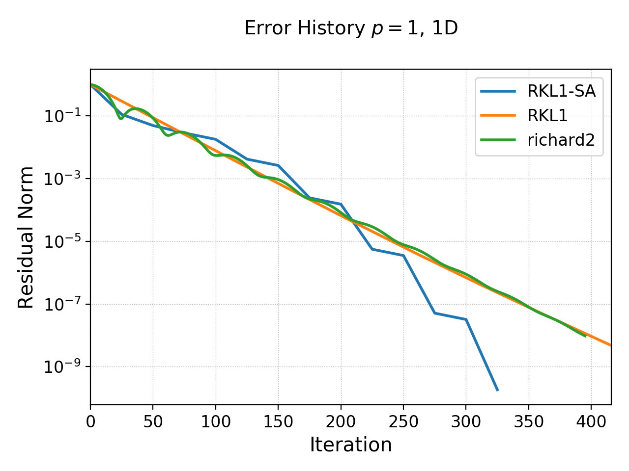
History of residual norm for \(p=1\), 1D \(64\) cell case for “RKL1+SA” (blue), “richard2” (green) and “RKL1” (orange) schemes. Note the exponential decay in errors, with the “RKL1+SA” further converging faster due to the sequence acceleration. The “richard2” scheme has some oscillatory mode (as can be seen from the dispersion relation also).

The convergence of the \(p=2\) scheme is shown in the following table.

Poisson solver convergence for 1D, \(p=2\) periodic BCs

\(N_x\)	\(l_2\)-error	Order	\(N_{RKL1}\)	\(N_{rich}\)
8	\(3.35174\times 10^{-4}\)		55	85
16	\(5.79245\times 10^{-6}\)	5.85	100	166
32	\(9.25562\times 10^{-8}\)	5.97	198	412
64	\(1.45406\times 10^{-9}\)	5.99	444	997

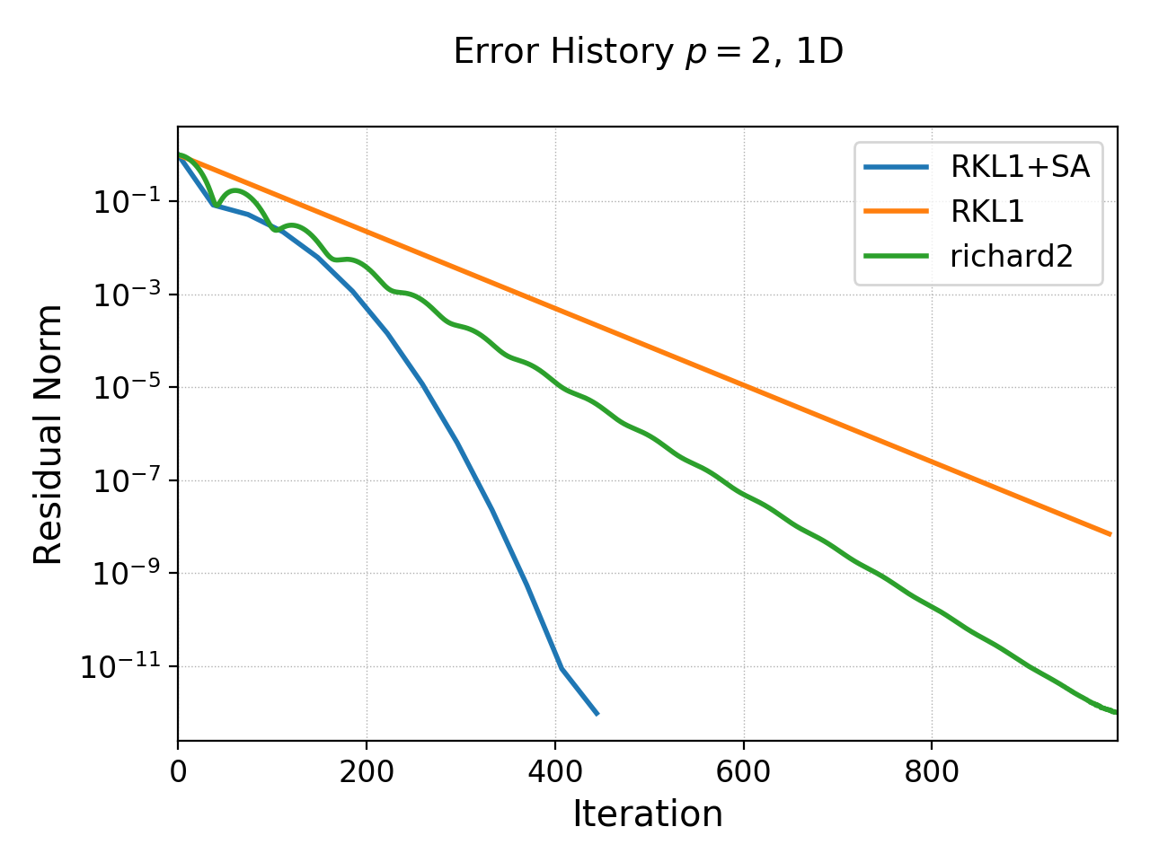
History of residual norm for \(p=2\), 1D \(64\) cell case for “RKL1+SA” (blue), “richard2” (green) and “RKL1” (orange) schemes. Note the exponential decay in errors, with the “RKL1+SA” further converging faster due to the sequence acceleration. The “richard2” scheme has some oscillatory mode (as can be seen from the dispersion relation also).

Convergence tests in 2D

For 2D convergence tests I used the source

\[ s(x,y) = -\frac{1}{N}\sum_{m,n} (m^2+n^2) \left[ a_{mn} \cos(mx) \cos(ny) + b_{mn} \sin(mx) \sin(ny) \right].\]

with \(x\in [0,2\pi]\) and \(y\in [0,2\pi]\) on a periodic domain. This source source is set in code as:

local initSource = Updater.ProjectOnBasis {
   onGrid = grid,
   basis = basis,
   evaluate = function(t, xn)
      local x, y = xn[1], xn[2]
      local amn = {{0,10,0}, {10,0,0}, {10,0,0}}
      local bmn = {{0,10,0}, {10,0,0}, {10,0,0}}
      local t1, t2 = 0.0, 0.0
      local f = 0.0
      for m = 0,2 do
         for n = 0,2 do
            t1 = amn[m+1][n+1]*math.cos(m*x)*math.cos(n*y)
            t2 = bmn[m+1][n+1]*math.sin(m*x)*math.sin(n*y)
            f = f + -(m*m+n*n)*(t1+t2)
         end
      end
      return -f/50.0
   end,
}

The exact solution for this problem is

\[ f_e(x,y) = \frac{1}{N}\sum_{m,n} \left[ a_{mn} \cos(mx) \cos(ny) + b_{mn} \sin(mx) \sin(ny) \right].\]

Gird size of \(8\times 8\), \(16\times 16\), \(32\times 32\), \(64 \times 64\) cells were used. The errors, convergence order and number of iterations to converge to a residual norm of \(10^{-8}\) are given below. Note that both the “RKL1” and “richard2” converge to the same \(l_2\)-norm error.

Poisson solver convergence for 2D, \(p=1\) periodic BCs

\(N_x\)	\(l_2\)-error	Order	\(N_{RKL1}\)	\(N_{rich}\)
\(8\times 8\)	\(1.31167\times 10^{-2}\)		44	81
\(16\times 16\)	\(9.07424\times 10^{-4}\)	3.85	90	157
\(32\times 32\)	\(5.8352 \times 10^{-5}\)	3.96	170	312
\(64\times 64\)	\(3.67363\times10^{-6}\)	3.99	352	624

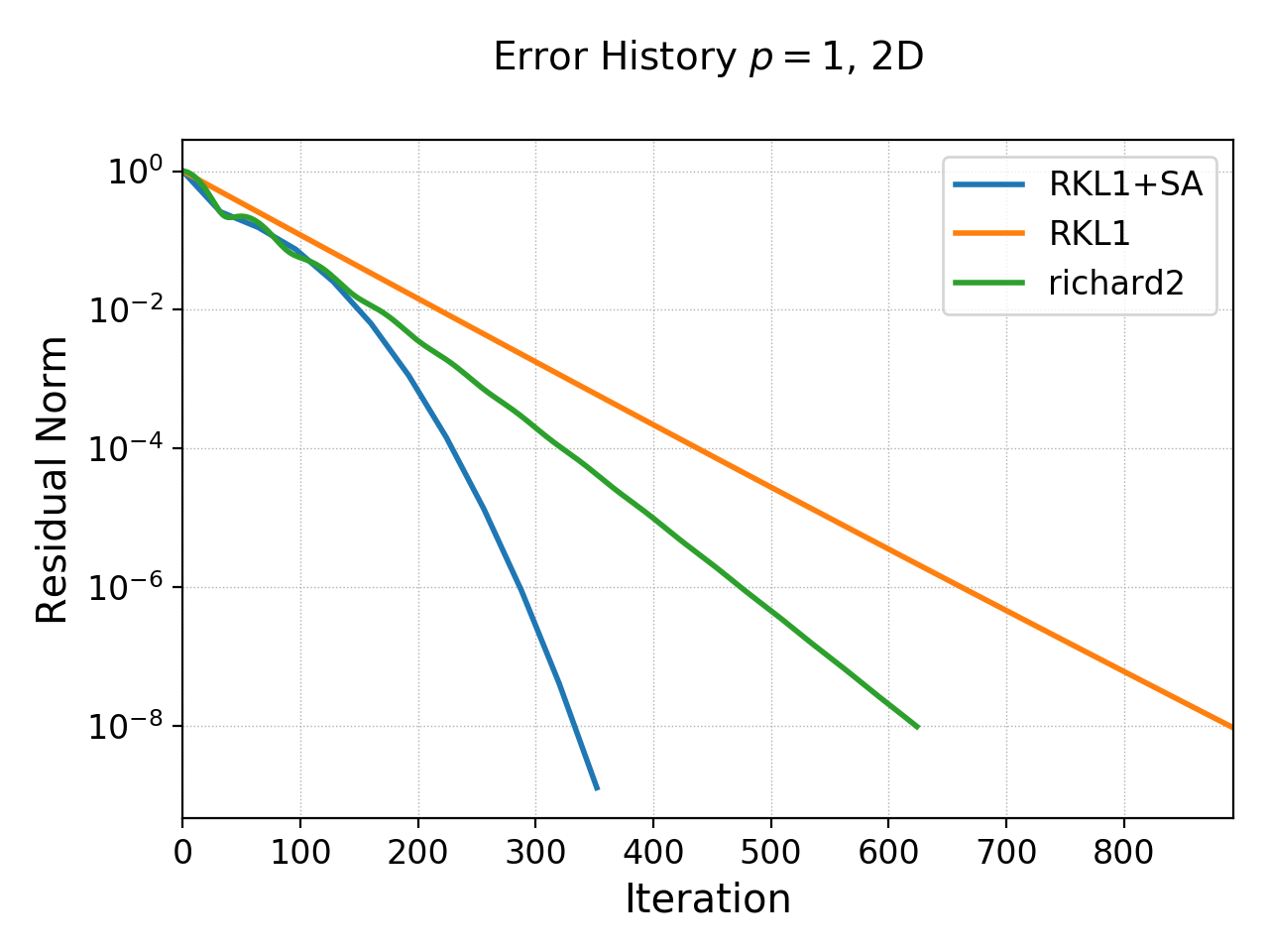
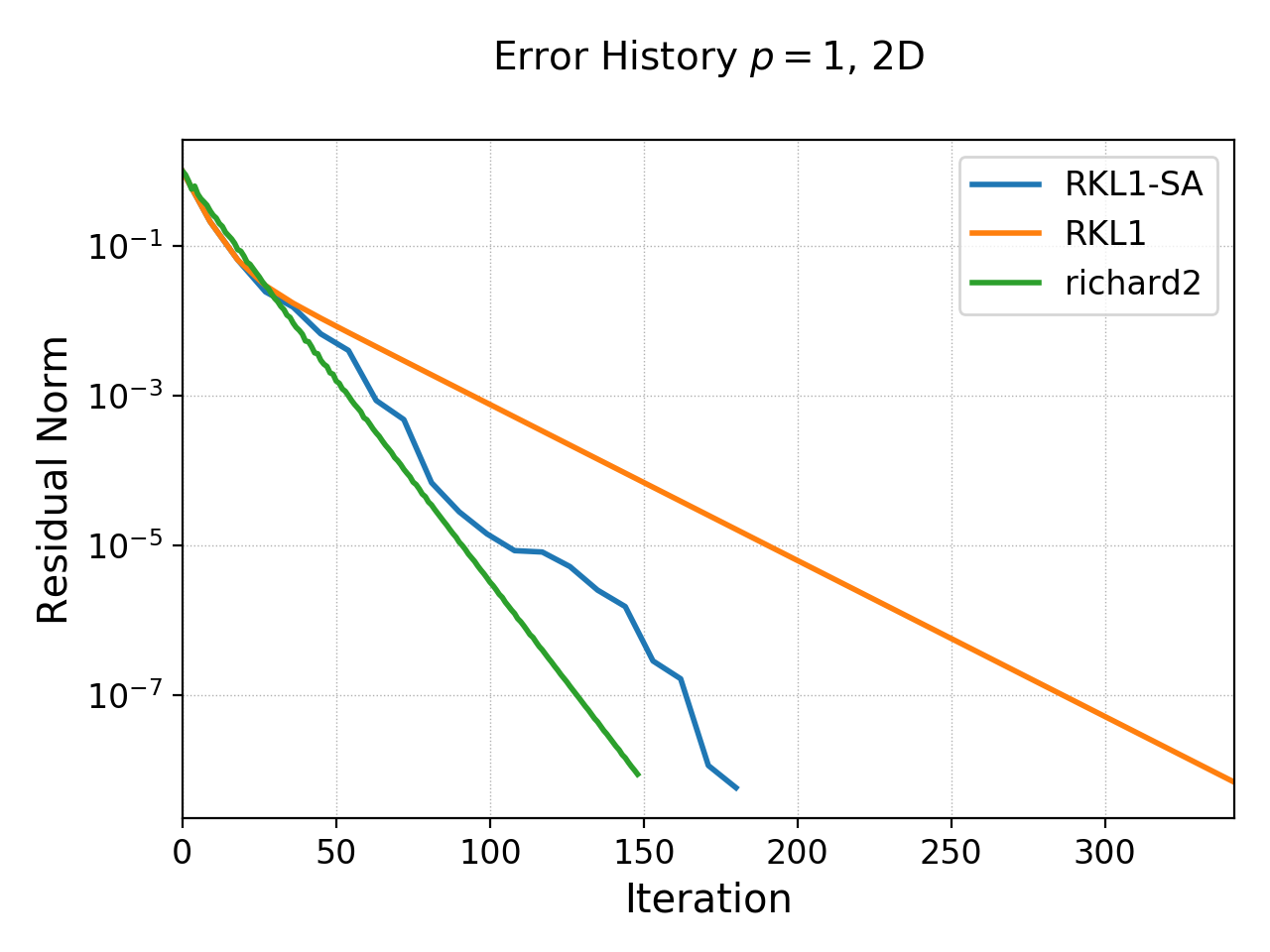
History of residual norm for \(p=1\), 2D \(64\times 64\) cell case for “RKL1+SA” (blue), “richard2” (green) and “RKL1” (orange) schemes. Note the exponential decay in errors, with the “RKL1+SA” further converging faster due to the sequence acceleration. The “richard2” scheme has some oscillatory mode (as can be seen from the dispersion relation also).

Poisson solver convergence for 2D, \(p=2\) periodic BCs

\(N_x\)	\(l_2\)-error	Order	\(N_{RKL1}\)	\(N_{rich}\)
\(8\times 8\)	\(1.98078\times 10^{-4}\)		96	132
\(16\times 16\)	\(3.42286\times 10^{-6}\)	5.85	130	261
\(32\times 32\)	\(5.47957 \times 10^{-8}\)	5.96	275	642
\(64\times 64\)	\(8.59271\times10^{-10}\)	5.99	600	1406

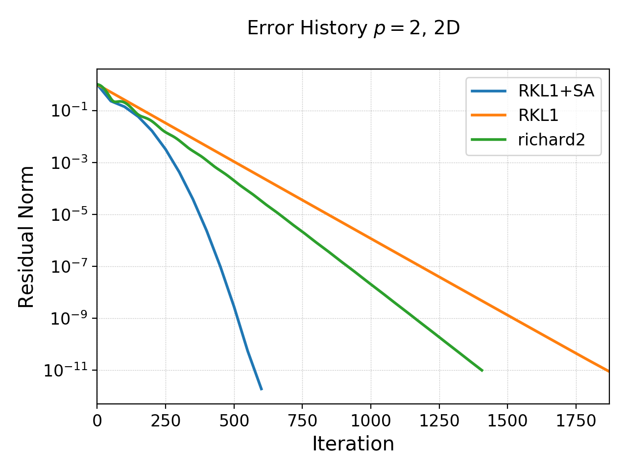
History of residual norm for \(p=2\), 2D \(64\times 64\) cell case for “RKL1+SA” (blue), “richard2” (green) and “RKL1” (orange) schemes. Note the exponential decay in errors, with the “RKL1+SA” further converging faster due to the sequence acceleration. The “richard2” scheme has some oscillatory mode (as can be seen from the dispersion relation also).

In the following plot the RDG solution is compared with the exact solution for the \(p=2\) case, showing the accuracy of the scheme on a coarse grid of \(8\times 8\) grid.

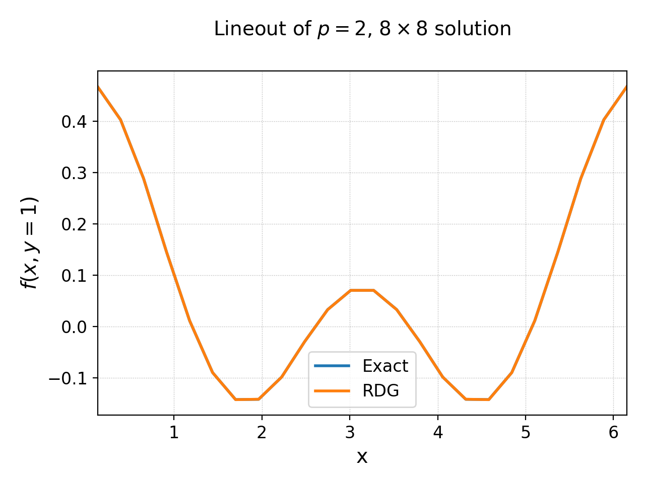
Lineout of RDG solution (orange) and exact solution (blue) for 2D \(8\times 8\) grid with \(p=2\) basis functions. The two curves essentially overlap, showing the accuracy of the RDG scheme for this problem.

Convergence tests in 3D

For 3D convergence tests I used the source

\[ s(x,y,z) = -\frac{1}{N}\sum_{m,n} (m^2+n^2+9) \left[ a_{mn} \cos(mx) \cos(ny) + b_{mn} \sin(mx) \sin(ny) \right]\sin(3z).\]

with \(x,y,z\in [0,2\pi]\) on a 3D periodic domain. This source source is set in code as:

local initSource = Updater.ProjectOnBasis {
   onGrid = grid,
   basis = basis,
   evaluate = function(t, xn)
      local x, y, z = xn[1], xn[2], xn[3]
      local amn = {{0,10,0}, {10,0,0}, {10,0,0}}
      local bmn = {{0,10,0}, {10,0,0}, {10,0,0}}
      local t1, t2 = 0.0, 0.0
      local f = 0.0
      for m = 0,2 do
         for n = 0,2 do
            t1 = amn[m+1][n+1]*math.cos(m*x)*math.cos(n*y)*math.sin(3*z)
            t2 = bmn[m+1][n+1]*math.sin(m*x)*math.sin(n*y)*math.sin(3*z)
            f = f + -(m*m+n*n+9)*(t1+t2)
         end
      end
      return -f/50.0
   end,
}

The exact solution for this problem is

\[ f_e(x,y,z) = \frac{1}{N}\sum_{m,n} \left[ a_{mn} \cos(mx) \cos(ny) + b_{mn} \sin(mx) \sin(ny) \right] \sin(3z)\]

Gird size of \(8\times 8\), \(16\times 16\), \(32\times 32\), \(64 \times 64\) cells were used. The errors, convergence order and number of iterations to converge to a residual norm of \(10^{-8}\) are given below. Note that both the “RKL1” and “richard2” converge to the same \(l_2\)-norm error.

Poisson solver convergence for 3D, \(p=1\) periodic BCs

\(N_x\)	\(l_2\)-error	Order	\(N_{RKL1}\)	\(N_{rich}\)
\(8\times 8\times 8\)	\(1.50795\times 10^{-1}\)		42	36
\(16\times 16\times 16\)	\(1.15276\times 10^{-2}\)	3.7	54	77
\(32\times 32\times 32\)	\(7.63856 \times 10^{-4}\)	3.9	77	157
\(64\times 64\times 64\)	\(4.84829\times 10^{-5}\)	3.98	154	316

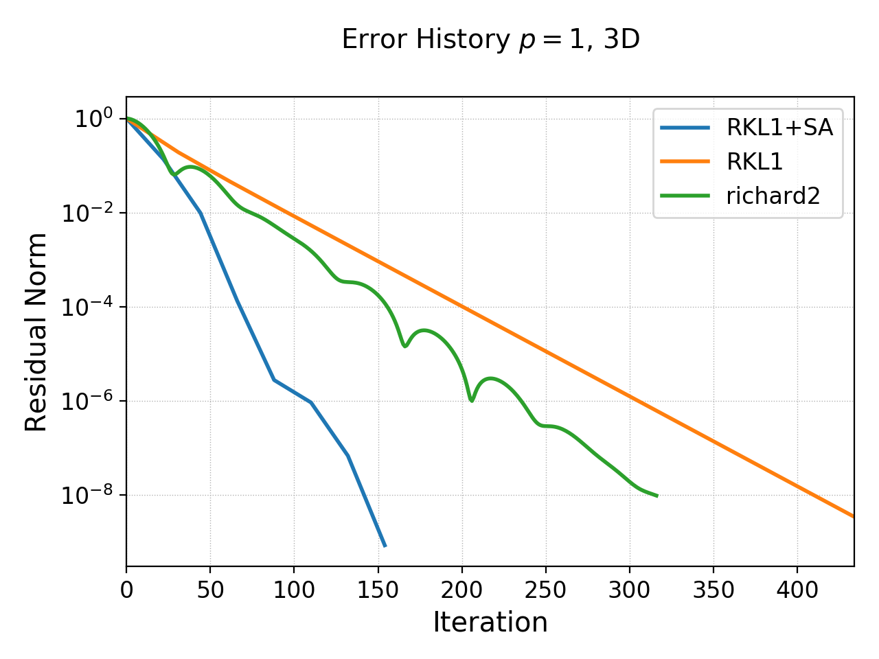
History of residual norm for \(p=1\), 3D \(64\times 64\times 64\) cell case for “RKL1” (blue) and “richard2” (orange) schemes. Note the exponential decay in errors, with the “RKL1” further converging faster due to the sequence acceleration. For the 3D case it seems there is persistent oscillatory modes which seem absent in 1D or 2D.

Though not shown here, a similar trend is seen for \(p=2\) 3D case and the scheme converges with 6th order accuracy.

Random source

To test if the sequence acceleration is effective simply because there are only a few wave modes in solutions used in the above test, I also tested the case in which the source is initialized randomly using the following code block:

local initSource = Updater.ProjectOnBasis {
   onGrid = grid,
   basis = basis,
   numQuad = 2*polyOrder+1,
   evaluate = function(t, xn)
      return math.random()
   end,
}

With this, the error history of the \(p=1\) basis code on \(16\times 16\) domain is show below for each of the three schemes.

History of residual norm for \(p=1\), 2D \(16\times 16\) cell case for “RKL1-SA” (blue), “richard2” (orange) and “RKL1” (orange) schemes. For this problem, the source (RHS) is initialized with random noise. Even though the “RKL1-SA” and “richard2” converge in about the same nunber of iterations, even in this extreme case the sequence acceleration does help reduce the number of iterations in about \(2\times\) from the “RKL1” case.

Note that even in this case the number of iterations scales linearly with the grid size. (I am not sure how to precisely initialize the source in a way that scaling with grid size can be properly studied. However, it does seem that the scaling holds in this case also).

How many iterations are needed?

Greg worked out an estimate of how many iterations would be needed by the second order Richardson scheme to get an error of \(10^{-n}\). The formula is:

\[N_{\rm iter} = \frac{1}{2} \ln(10^n) \left( \frac{\sqrt{N_d} (p+1) N_{\rm cells}}{\pi} +1 \right)\]

where \(p\) is the polyOrder, \(N_d\) is the dimension of the domain, and \(N_{\rm cells}\) are the number of cells in each direction (assuming a square domain with same number of cells in each direction). The following table shows the iterations computed from this formula and obtained using the ‘richard2’ scheme.

Number of expected iterations to converge to \(10^{-n}\) (\(n\) between 8 and 9) compared to actual iterations

Grid	polyOrder	\(N_{\rm iter}\)	\(N_{\rm gkyl}\)
\(16\)	1	106	101
\(16\times 16\)	1	146	148
\(16\)	2	168	171
\(16\times 16\)	2	234	241

Given this data is seems that IterPoisson is converging in a near-ideal manner.

Some concluding notes

It seems that the iterative Poisson solver is working well, and both the schemes converge with the best possible scaling for a local (3-point) iterative scheme. Multigrid schemes may scale better and be faster for large problems, but a side-by-side comparison remains to be done. Some concluding notes follow.

• The sequence acceleration implemented for the “RKL1” scheme makes it converge faster than the “richard2” scheme as well as without the sequence acceleration. The same sequence acceleration scheme does not work for “richard2” scheme, probably due to the presence of the oscillatory modes. Perhaps there is a way to apply such an acceleration to the “richard2” scheme also.

• Although the “RKL1” consistently outperforms the “richard2” scheme, the parameters are hard to choose and significant experimentation is needed. (Though the parameters are geometry dependent and do not depend on the source term). Hence, for now, “richard2” scheme is easier to use. Auto-selecting the parameter remains ongoing research. (A hint here is that once one determines the parameter for a given resolution then the parameters for doubling the grid in each direction are easy to determine).

• Compared to a direct solver, the iterative solvers are significantly faster for even modest size problems. For example, for \(16\times 16\times 16\), \(p=1\) problem the iterative solver is about 600x faster! (The number of degrees of freedom are \(16\times 16\times 16\times 8 = 32768\)) The bulk of the time is spent in the LU factorization. Further, even though the matrix is sparse, the LU factor are not and storing these may be an issue. However, for small problems for which the factorization can be done once and the LU factors stored, the direct solver can be faster as for each solve (after factorization) only a back-substitution is needed.

• The iterative solver works in parallel. The \(64\times 64\times 64\), \(p=1\) problem runs about 1.98x faster on 2 cores and 3.4x faster on 4 cores.

• Further improvements are possible, for example, applying some preconditioner to the system. This could reduce the cost further at the expense of a complicated implementation.

References

Meyer2014

C.D. Meyer, D.S. Balsara, T.D. Aslam. “A stabilized Runge–Kutta–Legendre method for explicit super-time-stepping of parabolic and mixed equations”. Journal of Computational Physics, 257 (PA), 594–626. http://doi.org/10.1016/j.jcp.2013.08.021, (2014).

Golub1961

G.H Golub, R.S. Varga. “Chebyshev semi-iterative methods, successive overrelaxation iterative methods and second order Richardson iterative methods”, Numerische Mathematik 3, 147–156. (1961)

Jardin2010

S. Jardin. “Computational Methods in Plasma Physics”, Chapman & Hall/CRC Computational Science Series (2010).

Nishikawa2007

H. Nishikawa. “A first-order system approach for diffusion equation. I: Second-order residual-distribution schemes”. Journal of Computational Physics, 227 (1), 315–352. http://doi.org/10.1016/j.jcp.2007.07.029 (2007)