JE8: Propagation into a plasma wave beach
A plasma wave beach is a slab configuration in which the density increases monotonically. An electromagnetic wave is pumped into the beach (hence the name wave beach). The wave frequency \(\omega\) is arranged such that at some location \(x=x_c\), \(\omega = \omega_p(x_c)\). At this location the electromagnetic wave suffers a cutoff and is reflected back towards the drive plane, creating a standing wave pattern.
In this entry this problem is simulated with Lucee. The plasma profile is selected as
where \(0<x<L\) is the domain and \(\delta t\) is a constant with units of time. The electromagnetic wave is driven by a current applied at the center of the last cell, i.e.,
where \(x_e = L-\Delta x /2\), where \(\Delta x\) is the cell size.
We pick \(\omega \delta t = \pi /10\). With \(L=1\) the cutoff location is \(x_c \approx 0.58\). We pick \(\delta t = L/100c\), where \(c\) is the speed of light. Further, the electron temperature is set to 1 eV and the ion fluid is not evolved, i.e., on the time-scale of the problem the ions are assumed to be immobile.
This problem is interesting as with conventional explicit FDTD methods a numerical instability occurs at cutoff and resonance layers. This means that implicit algorithms are needed to simulate such problems. See the paper by David Smithe [Smithe2007] for an algorithm in which the plasma is treated as a cold linear medium that is evolved implicitly to avoid the instability.
EM wave propagation in vacuum
In the first test the problem is simulated without the plasma. This is essentially a test to ensure the EM wave propagation works correctly with the current source. Simulations are performed by setting \(J_0=1\times 10^{-12}\) and run to \(t=5\) ns. Grids with 100 and 200 cells are used. Results are shown below. Note that although the solutions are smooth limiters need to be applied as the sudden appearance of \(E_y\) due to the current source causes a shock that propagates into the ghost cell, which in turns spoils the interior solution. The limiters are what cause the maxima in the solutions shown below to get slightly flattened.

Electromagnetic wave propagation in vacuum driven by a current source in the last cell. Shown here is the electric field \(E_y\) at \(t=2.5\) ns (top) and \(t=5.0\) ns (bottom) for 100 cells [s65] (red line) and 200 cells [s66] (black line). In the upper panel the electromagnetic wave has not yet propagated through the domain.
Wave propagation into a plasma beach
In this set of simulations wave propagation into the plasma beach is presented. The time-step for this simulation needs to be small enough to resolve the plasma frequency. Several simulations were performed: with 100, 200, 400 and 800 grid cells. The transverse electric field, \(E_y\) is plotted as a function of space and time below.
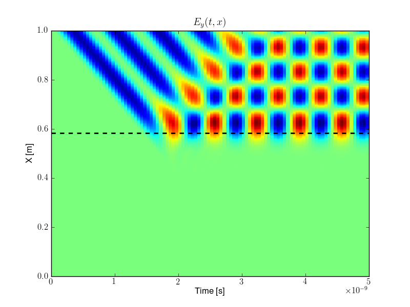
Electromagnetic wave propagation in a plasma beach driven by a current source in the last cell. This simulation [s69] was run on a 400 cells. Shown here is the electric field \(E_y\) as a function of time (increasing towards the right) and space (top of the figure is the right edge). The dashed black line shows the plasma cutoff (\(\omega_p(x) = \omega\)). The EM wave propagates into the plasma and reflects off the cutoff layer, interfering with the incoming wave. Evanescent waves propagating into the cutoff region are also visible.
The convergence of the solution with increasing grid resolution is shown below. It is seen that the 100 cell resolution is very diffuse. The reason for this is that the small CFL number (0.1) causes significant diffusion in the wave-propagation scheme.
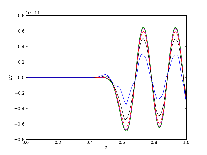
Comparison of \(E_y\) for different grid sizes. Show are results from 100 cells (blue) [s67], 200 cells (black) [s68], 400 cells (red) [s69], 800 cells (magenta) [s70] and 1600 cells (green) [s71]. The lower resolution simulations show significant diffusion as the wave-propagation scheme can not be run to the allowed CFL number as the plasma-frequency needs to be resolved.
Conclusions
This simulation shows that radio-frequency EM wave propagation into a plasma cutoff can be simulated with the wave-propagation scheme in a stable manner. Note that the plasma frequency needs to be resolved. This constraint can be quiet severe and a way around this would be advance the source terms (semi-) implicitly. Another option would be to treat the electrons as a cold linear dielectric medium (in the spirit of Smithe). Of course, this would exclude non-linear electron physics.
The fact that the wave-propagation scheme is so diffusive for time-steps much smaller than allowed by the CFL number is a significant disadvantage. High-order schemes are not so sensitive to CFL numbers and should be of value here. Another option would be to evolve the fields and fluid with different time-steps and using implicit source advance to couple them.
References
- Smithe2007
David N Smithe, “Finite-difference time-domain simulation of fusion plasmas at radiofrequency time scales”, Physics of Plasmas, 14, Pg. 056104 (2007).