JE34: Multi-moment multifluid linear dispersion solvers
Contents
Introduction
In this note I benchmark and document the multi-moment multifluid dispersion solver tool in Gkeyll. This solver allows arbitrary number of species, each of which can be either an isothermal fluid, a five-moment fluid or a ten-moment fluid. The fields can be computed from Maxwell equations or Poisson equations, with the option of some species “ignoring” the background fields. Certain forms of closures, including non-local Hammett-Perkins Landau fluid closures can be used.
For the list of equations and a brief overview of the algorithm used, please see this technical note. Essentially, the key idea of this algorithm is to convert the problem of finding the dispersion relation to an eigenvalue problem and then use a standard linear algebra package (Eigen in this case) to compute the eigensystem. This allows great flexibility as there is no need to directly find complex nonlinear polynomial roots or even formulate the dispersion relation explicitly. I note that this technique was described in my 2008 paper on the ten-moment model [Hakim2008]. Since then, it has been significantly developed and used by Hausheng Xie and others. See, for example [Xie] and references therein. As far as I know, however, the inclusion of the ten-moment model and Landau closures is unique to Gkeyll.
Eventually, the goal is to perform a careful comparison of the linear physics contained in the ten-moment system (especially with various Landau and other simplified closures) with full kinetic equations. Other applications are to computing initial conditions that excite specific modes, computing RF wave-propagation and potential extension to retain quadratic nonlinearities to allow study of wave-wave scattering/coupling physics.
Note on running the dispersion solver tool
To run the tool create an input file (Lua script, see examples below in various figure captions) and run it as:
gkyl multimomlinear -i inp.lua
This will create a output file with the eigenvalues stored in a Gkeyll “DynVector” object. For each element in the dynvector, the first three components are the components of the wave-vector and the rest the corresponding \(\omega_n(\mathbf{k})\) with real and imaginary parts stored separately (next to each other). You can plot the real part of the frequencies as function of wave-vector (say \(k_x\)) as:
pgkyl -f inp_frequencies.bp val2coord -x0 -y 3::2 pl -s -f0 --no-legend --xlabel "k" --ylabel "$\omega_r$"
And the imaginary parts as:
pgkyl -f inp_frequencies.bp val2coord -x0 -y 4::2 pl -s -f0 --no-legend --xlabel "k" --ylabel "$\omega_i$"
Often, it is useful to plot the eigenvalues in the complex plane (real part on X-axis and imaginary part on the Y-axis). For this do:
pgkyl -f inp_frequencies.bp val2coord -x3::2 -y 4::2 pl -s -f0 --no-legend --xlabel "$\omega_r$" --ylabel "$\omega_i$"
Note that the frequencies are not outputed in any particular
order. Hence it is not possible to easily extract a single “branch” of
the dispersion relation from the output. Please see pgkyl help to
understand what the val2coord and pl (short for plot) do
and how to use them.
The boolean flag calcEigenVectors can be set to true to
optionally compute the eigenvectors. These are stored in a
CartField object.
Waves in a uniform plasma
In the first test I look at the problem of waves in a uniform plasma. The first test assumes the plasma is composed of cold electrons and ions (\(m_i/m_e = 25\)) with the background magnetic field \(\mathbf{B}_0 = (1.0, 0.0, 0.75)\) transverse to the wave-vector pointing in the X-direction . The following plot shows the various plasma waves that appear in the system.
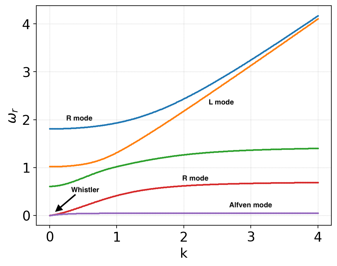
Waves in a cold magnetized plasma, with wave-vector transverse to the background magnetic field. Seen are the right (R) and left (L) polarized modes that asymptote to light waves at large \(k\). Also seen the second branch of the R mode which contains the Whistler mode at low-\(k\) and also the Alfven mode. See input file iso-1-wave.
In the next problem I use the five-moment model with a finite pressure \(p = 0.1\) for both electrons and ions. The dispersion relation is compared to the corresponding cold case in the following plot.
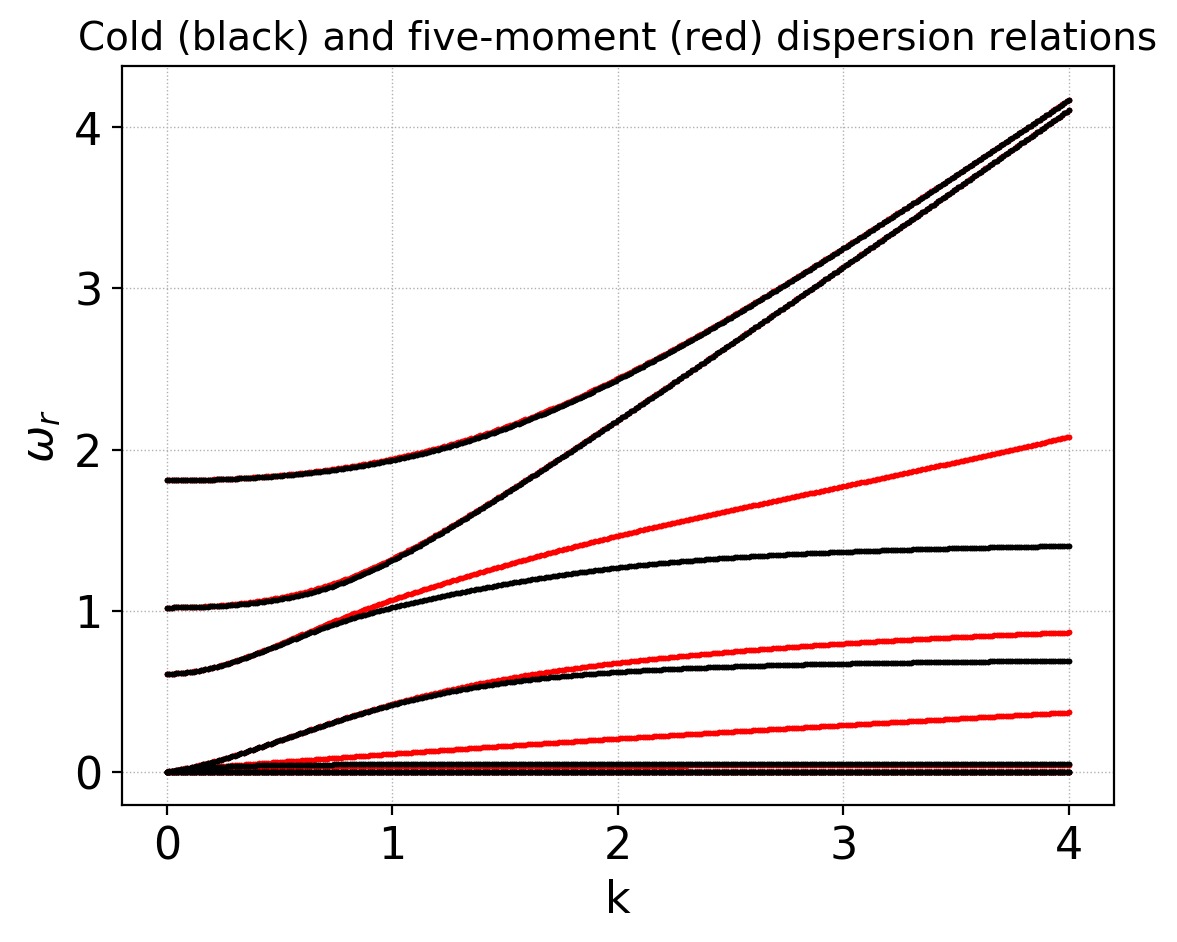
Waves in a cold (black) and five-moment finite-pressure (red) magnetized plasma, with wave-vector transverse to the background magnetic field. The finite pressure effect changes the sound-wave mediated branches, allowing them to propagating at high \(k\). See input file 5m-1-wave.
For the next test I use the ten-moment model with a diagonal pressure tensor \(P_{xx} = P_{yy} = P_{zz} = 0.1\) and all other components set to zero. This gives the same scalar pressure as the previous five-moment test. The ten-moment model has a a lot of modes. To illustrate the differences between five-moments the following plot shows the high-frequency branches of the dispersion relation. Note the existence of two cyclotron harmonics marked with \(\omega_{ce}\) and \(2 \omega_{ce}\) in the plot. These are missing in the five-moment model. Also, the R- and L-mode structure is different, with the lower cyclotron harmonic transitioning to the L-mode and the upper cyclotron harmonic to the R-mode at larger \(k\) values.
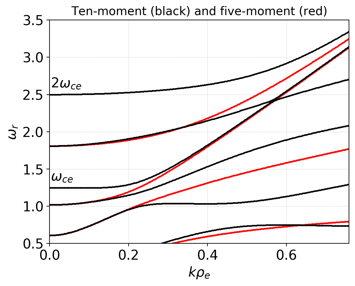
Comparison of high-frequency branches of the dispersion relation for ten-moment (black) and five-moment (red) models. The ten-moment model contains the first two electron cyclotron harmonics which transition to the L- and R-mode at higher \(k\). See input file 10m-1-wave.
The following plot shows the low-frequency branches of the ten-moment model compared to the five-moment model. Again, the two ion cyclotron harmonics are seen as well as the various ion acoustic mediated branches.
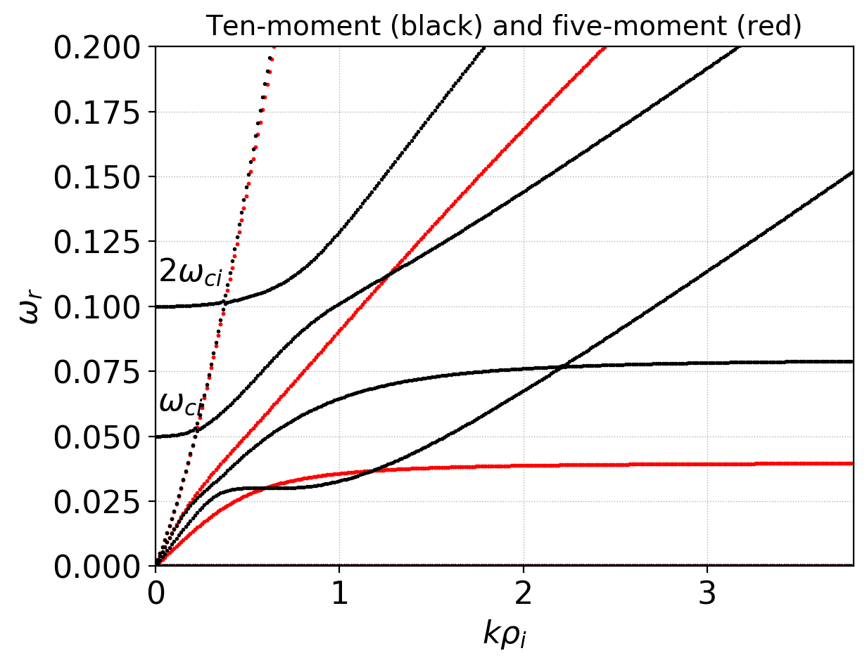
Comparison of low-frequency branches of the dispersion relation for ten-moment (black) and five-moment (red) models. The first two ion cyclotron harmonics are seen. See input file 10m-1-wave.
The tests in these sections were done without any closures, and in particular, without Landau closures. In the kinetic system many of the modes seen above are damped.
The Buneman instability
In the next series of tests various instabilities are used as benchmarks. First, consider the Buneman instability which was studied extensively in JE33. Consider a one-dimensional, electrostatic, collisionless plasma in which the electrons are drifting with respect to cold ions with speed \(V_0\) much larger than the electron thermal speed, i.e. \(V_0 \gg v_{the}\). In this case an electron perturbation couples to ion plasma oscillations, leading to an electrostatic instability called the Buneman instability. The following plot shows the growth rate of the instability for various wave-numbers for several different mass ratios. Note that this figure is identical to the one presented in JE33, giving confidence in the correctness of the linear dispersion solver implementation.
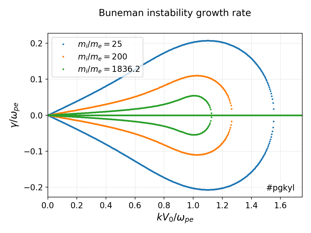
Growth rate as a function of \(k\) for various ion-electron mass ratios: \(m_i/m_e = 25\) (blue), \(m_i/m_e = 200\) (orange) and \(m_i/m_e = 1836.2\) (green). The instability grows slower with increasing mass ratio. For full study of this problem, including nonlinear kinetic simulations, see JE33. Also see tool input file for the \(m_e/m_e = 25\) case iso-2-bune.
To see which modes actually grow, the follow plot shows the spectrum of the modes in the complex plane for the \(m_i/m_e = 1836.2\) case. Only a very narrow range of low-frequency modes grow, while the higher frequency modes merely oscillate.
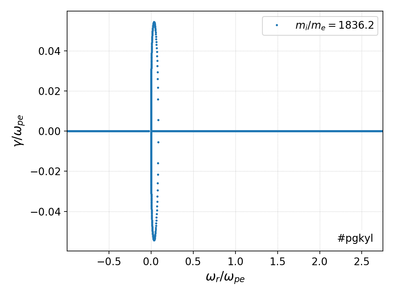
Spectrum of the modes in the complex plane for the Buneman instability. This plot shows that only the very low frequency modes grow, while the higher-frequency modes remain purely oscillating.
The Electron Cyclotron Drift Instability (ECDI)
The Electron Cyclotron Drift Instability (ECDI) is an electrostatic current-driven instability that arises due to \(\mathbf{E}\times\mathbf{B}\) motion of electrons. In the typical setup the ions are unmagnetized and hence do not contribute an \(\mathbf{E}\times\mathbf{B}\) current. (Note that in general there is no net \(\mathbf{E}\times\mathbf{B}\) current in an infinite plasma. However, in some situations it is possible that the ions never complete a gyroperiod and hence the ion currents are never set up). The ECDI is considered a mechanism of anomalous electron transport in Hall thrusters.
In the first set of simulations the electrons and ions are treated as isothermal fluids. The background electric field is set to \(E_y = 0.2\) and the background magnetic field to \(B_z = 1.0\). The growth of the instability vs \(k\) is shown below. The instability is active only for a small range of wave-numbers. Further, increasing mass-ratio reduces the growth rate and the range over which the instability is active.
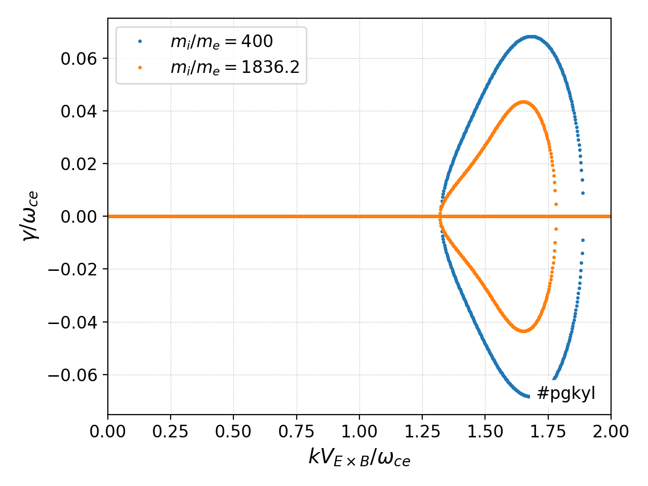
Growth rate vs \(k\) for the ECDI for a \(E\times B\) velocity of 0.2 for mass ratio of 400 (blue) and 1836.2 (orange). The instability is active for a narrow range of wave-numbers. The growth reduced with increasing mass ratio. See iso-ecdi-2 for an input file for the \(m_i/m_e = 1836.2\) case.
As for the Buneman instability, in the isothermal limit the instability only grows for low-frequency modes. See below.
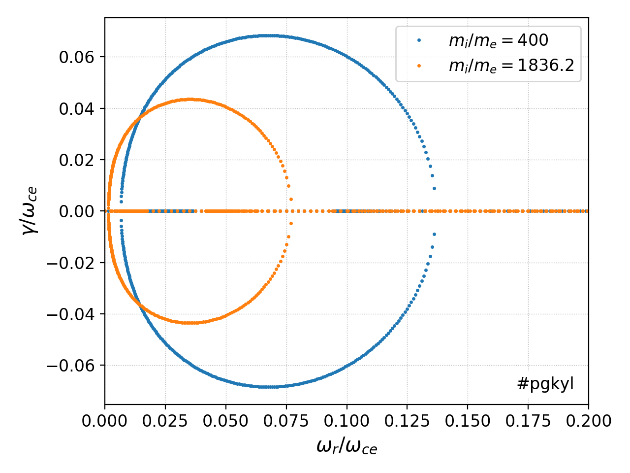
Spectrum of the modes in the complex plane for the ECDI. This plot shows that only the very low frequency modes grow, while the higher-frequency modes remain purely oscillating.
The real part of the dispersion relation is shown in the following plot for the \(m_i/m_e = 400\) case. The unstable modes are colored in red in the figure.
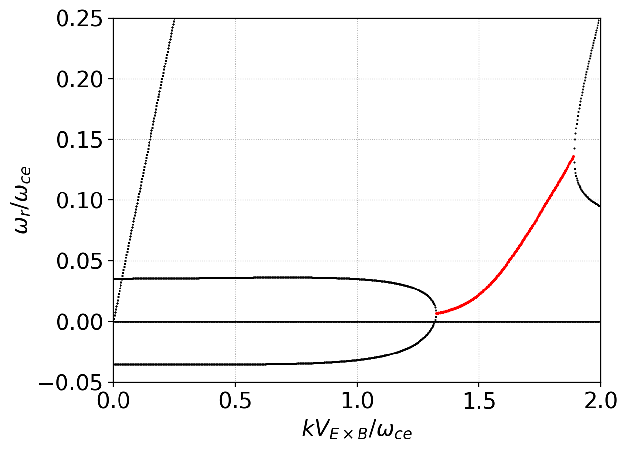
Real part of the dispersion relation for ECDI with isothermal fluids for the \(m_i/m_e = 400\) case. Marked in red are the unstable modes. As also seen in the above figures, only a very narrow range of modes are unstable.
We can also look at the ECDI with the ten-moment model. Here, due to the second cyclotron harmonic there is a second unstable branch that appears at even higher \(k\). However, at least for the parameters used here, the second mode grows more slowly, showing that in this setup the shorter \(k\) modes will be dominant.
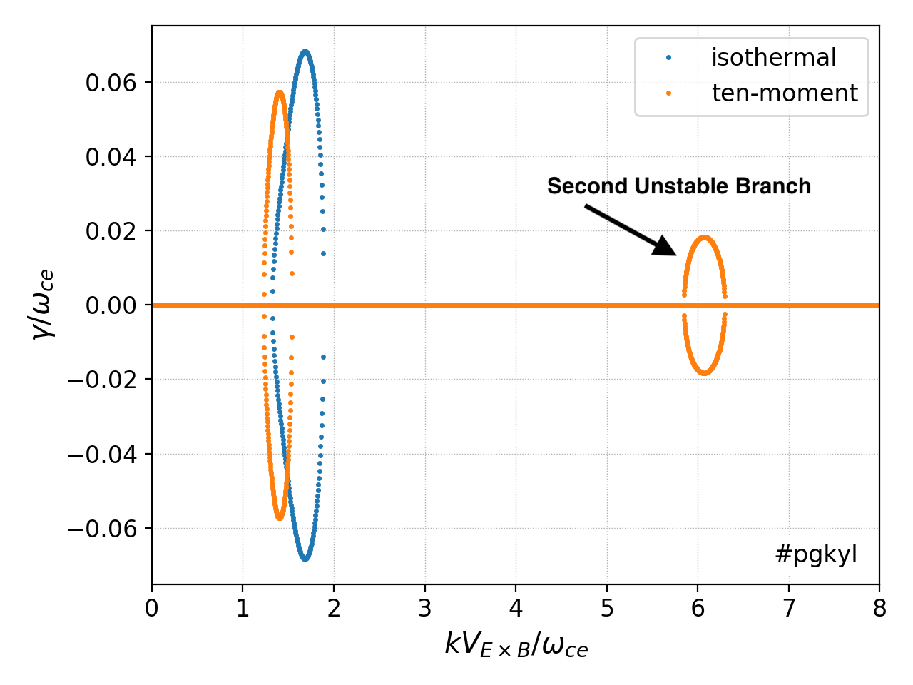
Growth rate of ECDI using the ten-moment model for both electrons and ions (orange) for mass-ratio \(m_i/m_e = 400\). Also shown for comparison are the growth rates from the isothermal case (blue). Note that there is a second unstable mode present in the ten-moment case due to the presence of the second harmonic. This mode, however, grows slower, indicating that the smaller \(k\) unstable modes will be dominant. See 10m-ecdi-1 for tool input file.
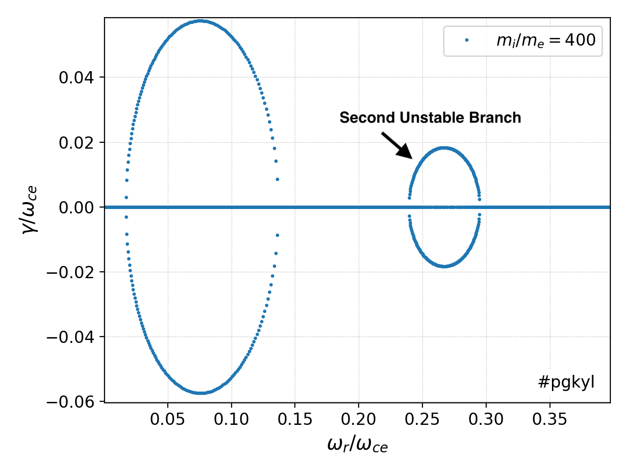
Spectrum of the modes in the complex plane for the ECDI using ten-moment model. This plot shows that only the very low frequency modes grow. Note the second set of unstable modes.
We can also look at the real frequencies of the various modes and identify the modes that grow. In this system there are huge number of modes but as seen from the above plots only those in a narrow range are unstable. The following plot shows a zoom into the low-frequency branches of the dispersion relation with the unstable modes colored in red. Again, note that there are two set of modes that are unstable, corresponding to the fact that there are two cyclotron harmonics included in the ten-moment model.
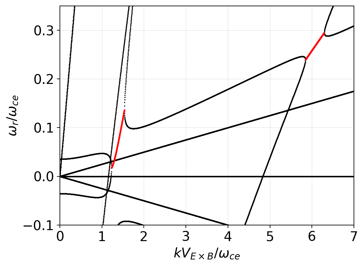
Low-frequency branches of the dispersion relation for ten-moment ECDI problem. Marked in red are the unstable modes that lead to the ECDI. Note the narrow region of \(k\) over which the instability is active. The two set of modes marked in red correspond to the two cyclotron harmonics included in the ten-moment model.
The Weibel instability
The Weibel instability is an electromagnetic instability that is excited when two counter-propagating electron beams are perturbed transverse to the direction of propagation. This instability leads to a growth of magnetic field. For a thorough kinetic study of the Weibel instability see our previous work [Skoutnev] and references therein. Shown below is the growth rate of the Weibel instability in the cold fluid limit, with the drift speed set to \(u_d = 1.0\).
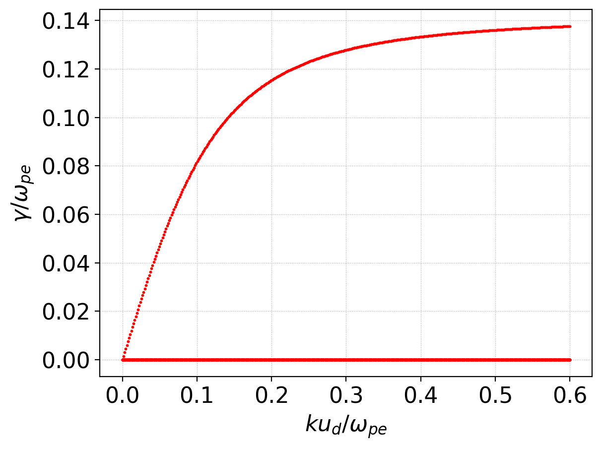
Growth rate of the Weibel instability in the cold fluid limit with drift speed of \(u_d = 0.1\). These values compare exactly with the analytical expression given in [Califano] Eq 12. See iso-weibel-1 for tool input file.
Note that for a full understanding of the Weibel modes one must use fully kinetic simulations. For example, in the warm case when \(u_d = v_{th}\) the isothermal fluid shows no growth, though the system is unstable in the kinetic regime. We can, however, study this warmer case with the ten-moment model that contains more physics than the isothermal model. For the cold case, the ten-moment model agrees exactly with the isothermal cold-fluid case. However, for the warm case in which isothermal model show no growth the ten-moment model shows an unstable mode. The growth rate for this is shown below. Also, shown in red dots are the growth rates from a kinetic calculation of the dispersion relation. The ten-moment models predicts the growth rate reasonably well for lower \(k\) modes but then deviates for higher \(k\). The kinetic and ten-moment comparisons get worse as the electron beams get warmer.
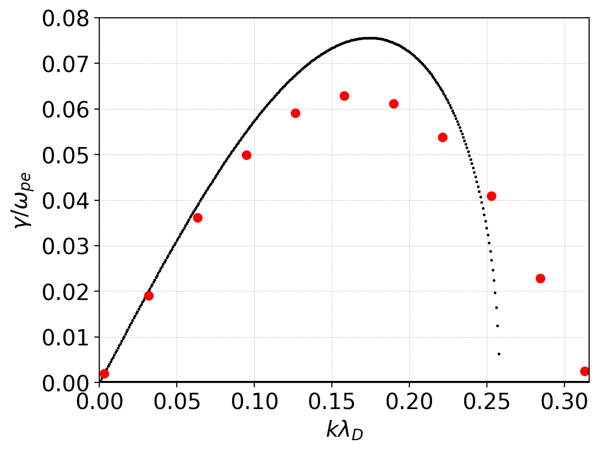
Growth rate of the Weibel instability with ten-moment model with drift speed \(u_d = v_{th}\). With these parameters the isothermal model does not show any growth. Also, shown in red dots are the growth rates from a kinetic calculation of the dispersion relation. (Code courtesy of Petr Cagas). The peak growth rates are about \(20\%\) higher in the ten-moment model. See 10m-weibel-2 for tool input file.
References
- Hakim2008
A.H. Hakim. “Extended MHD Modelling with the Ten-Moment Equations”. Journal of Fusion Energy, 27 (1-2), 36–43. http://doi.org/10.1007/s10894-007-9116-z
- Xie
H. Xie, Y. Xiao. “PDRK: A General Kinetic Dispersion Relation Solver for Magnetized Plasma”. Plasma Science and Technology, 18 (2), 97–107. http://doi.org/10.1088/1009-0630/18/2/01
- Skoutnev
W. Skoutnev, A. Hakim, J. Juno, J.M TenBarge, “Temperature-dependent Saturation of Weibel-type Instabilities in Counter-streaming Plasmas”. The Astrophysical Journal Letters, 872(2), 2019. http://doi.org/10.3847/2041-8213/ab0556
- Califano
F. Califano, F. Pegoraro, S.V. Bulanov. “Spatial structure and time evolution of the Weibel instability in collisionless inhomogenous plasmas”. Physical Review E, 56(1), 1–7, 1997