JE31: Enhancers or anti-limiters for robust evolution of distribution functions
Note
This note is written in conjunction with Greg Hammett of PPPL.
Contents
Introduction
The distribution function of particles is a non-negative scalar function. That is \(f(\mathbf{x},\mathbf{v},t)\ge 0\). However, there is no guarantee that a numerical scheme will preserve this property. In the discontinuous Galerkin (DG) scheme the distribution function in each cell is expanded in polynomial basis functions. Standard DG scheme does not guarantee that the value of the distribution function inside all cells remains positive. Even the positivity of the cell average is not guaranteed (for higher than piecewise constant basis functions) unless significant care is taken.
Standard positivity limiting, for example, the Zhang-Shu algorithm described in [Zhang2011], can’t be used for evolution of kinetic equations, when applied as a post-processing step. The reason for this is that the algorithms that change the moments of the distribution function (while maintaining cell averages) will change the particle energy. (The energy conservation in kinetic system is indirect, unlike fluid systems in which one evolves an explicit energy equation). Hence, use of such “sub-diffusion” based positivity schemes should be minimized or avoided altogether, if possible.
In the original Zhang-Shu algorithm, in which sub-cell diffusion is added in the spatial operator only, unless something is done to bound slopes (like monotonicity limiters) the slopes will grow in an unbounded manner. Hence, the Zhang-Shu algorithm needs an additional monotonicity or sub-cell diffusion post-processing step, again changing the particle energy.
In this note we show how one can obtain a positivity preserving DG scheme (defined precisely below), significantly improving robustness of algorithms for gyrokinetics and fully kinetic DG solvers. Although the use of anti-limiters does not completely eliminate the need to apply additional sub-cell diffusion, it significantly reduces the need for such additional corrections, dramatically improving the energy conservation property of the scheme.
(As additional diffusion can be applied to volume integrals also, in which case it may be possible to completely eliminate the need to apply sub-cell diffusion. This diffusion does not change the energy in gyrokinetic equations).
Exponential reconstruction
The DG scheme, in a sense, does not tell us the solution, but only the moments of the solution in each cell. However, we know that an infinite number of functions can be constructed from given set of moments. For problems in plasma physics we know that locally, the solution should be well approximated by a exponential function, which, by definition, is positive. Hence, one can take the moments (expansion coefficients) from a DG scheme and construct a positive function (exponential) with the same moments, and treat that as the solution. This can be thought of as a definition of a positivity preserving scheme: i.e. if one can construct a function that is positive everywhere in the cell, then the scheme is called positivity preserving. Note that we do not actually need to construct the positive function, but simply show that some such function exists.
Then, the question becomes: given a set of moments, is it always possible to reconstruct an exponential? Or, are there some bounds on the moments that permit the construction of an exponential?
Consider a distribution function \(f(x) = f_0 + f_1 x\), for \(x\in[-1,1]\). Now, consider finding a new function \(g(x) = \exp(g_0 + g_1 x)\) such that the moments match. We will write this as
(Note this is not strict equality, only equality in the \(L_2\) sense, that the projection of both sides on a set of basis functions are the same). Taking moments with the definition \(\langle \cdot \rangle\equiv \int_{-1}^1 (\cdot)\thinspace dx\), we get
where \(g_R = e^{g_0+g_1}\) and \(g_L = e^{g_0-g_1}\). This is a coupled set of nonlinear equations for \(g_1\) and \(g_2\) and can be solved with the following Python code
from numpy import *
import scipy.optimize

def func(an, f0, f1):
    a0 = an[0]; a1 = an[1]
    rhs0 = (exp(a1+a0) - exp(a0-a1))/a1
    rhs1 = ((a1-1)*exp(a0+a1) + (a1+1)*exp(a0-a1))/a1**2

    return rhs0-2*f0, rhs1-2.0/3.0*f1

# compute g0 and g1 for f0=1, f1=1.0 with initial guess 1.0, 0.01
aout = scipy.optimize.fsolve(func, [1.0, 0.01], args=(1.0, 1.0))
g0 = aout[0] # -0.18554037586019248
g1 = aout[1] # 1.0745628995369829
To gain some insight use the first equation to express \(g_1\) and substitute this in the second equation to solve for \(g_R\), for example, to get
This shows that as \(f_1 \rightarrow 3 f_0\), \(g_R \rightarrow \infty\). Similarly, we can show that as \(f_1 \rightarrow -3 f_0\), \(g_L \rightarrow \infty\), hence showing that we must have the bound
Defining \(r \equiv f_1/f_0\) we see that for a exponential reconstruction to exist, we must have \(|r| \le 3\). Hence, in 1D for piecewise linear basis functions, we say that the scheme is positivity preserving if \(f_0>0\) and \(|f_1|/f_0 \le 3\).
The figure below shows \(g_L\) and \(g_R\) as a function of \(r\).
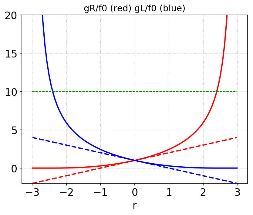
Exact nonlinear fits of \(g_R/f_0\) (solid red), \(g_L/f_0\) (solid blue) as a function of \(r=f_1/f_0\). Also shown are the cell edge values computed from \(f_0(1 \pm r)\) (dashed red/blue). The exponential fit, even though has the same moments as the linear function, always gives larger edge values than those computed from the linear function. The green dashed line is a “out-flow flux capping” limit, explained further below.
Enhancers or anti-limiters
Consider the the advection equation in 1D
where \(u>0\). A DG scheme is derived here in the standard way. Let \(\varphi\) be a test function in some function space. Let \(I_i\equiv [x_{j+1/2},x_{j-1/2}]\) be a cell in the grid, and let \(x_j \equiv(x_{j+1/2}+x_{j-1/2})/2\). Then, multiplying the advection equation by \(\varphi\) and integrating by parts one gets the discrete weak-form
where now \(f(x,t)\) lies in the discrete function space, \(\hat{F}_{j\pm1/2}\) are numerical fluxes at cell interfaces and the \(\varphi(x_{j\pm1/2}^\mp)\) indicate evaluation of the test functions just inside the cell \(I_{j}\). The numerical fluxes are computed using simple upwinding as
where \(f_{j\pm1/2}^{\mp}\) are the evaluation of the discrete distribution function just inside the cell \(I_j\).
For a piecewise linear DG scheme \(\varphi \in \{1, 2(x-x_j)/\Delta x\}\) is selected, and the solution is expanded in each cell \(f_j(x,t) = f_{j,0} + 2f_{j,1}(x-x_j)/\Delta x\). The update formula for piecewise linear case can now be derived by putting each of the \(\varphi\) in turn to get
where \(\sigma \equiv u\Delta t/\Delta x\).
In a standard DG scheme we would compute the edge values needed in the numerical flux with \(\hat{f}_{j+1/2}=f_{j,0}+f_{j,1}\) and \(\hat{f}_{j-1/2}=f_{j-1,0}+f_{j-1,1}\). Instead, in our enhancer or anti-limiter based scheme we compute the edge values as
where \(g_L\) and \(g_R\) are the edge values computed from an exponential reconstruction (or an approximation to it). (Need to explain why enhancement is better than standard DG scheme.)
The complete 1D scheme is hence:
At each step, given \(f_0\) and \(f_1\) compute estimates of \(g_L\) and \(g_R\)
Cap the outgoing flux such that in a step or RK stage the cell average does not go negative (i.e. ensure that we don’t remove so many particles from a cell in a single step such that the distribution function goes negative). The first of the update equations shows that this means that we must cap \(g_R \le f^n_0/\sigma\). This is the green dashed line in the above plot.
Note that this scheme guarantees that the cell average will remain positive, however, does not guarantee that the cell slope bound of \(|f_1|/f_0 \le 3\) will be maintained.
Extension to multiple dimensions
In higher dimensions we can take one of two approaches to construct an anti-limiter. Either we can attempt to reconstruct a multi-dimensional exponential function from the expansion coefficients, or use a dimension-by-dimension reconstruction, reusing the 1D reconstruction scheme multiple times. We use the latter approach in the following tests.
(Need to explain the 2D algorithm in detail, and why it seems to work so well)
Sub-cell diffusion
Even with anti-limiters the scheme does not guarantee that the slope bounds will be preserved, even in 1D. In 2 or higher dimensions determining slope bounds is a very hard problem and hence, instead, some other means are needed to ensure slope bounds are maintained. (Description of sub-cell diffusion scheme)
Convergence tests in 2D
To check convergence of the scheme, I initialize a simulation with a Gaussian initial condition
where \(r^2 = (x-x_c)^2+(y-y_c)^2\) and \(x_c, y_c\) is the domain center coordinates. Simulations are performed with polyOrder 1 basis functions on \(1\times 1\) domain with a sequence of grids with \(8\times 8\), \(16\times 16\) and \(32\times 32\) resolution. The time-step for each simulation is held fixed. The Gaussian propagates diagonally and, due to periodic boundary conditions, returns back to the origin at the end of simulation.
To compute error we use the measure
As seen below DG scheme demonstrates super-convergence in this norm.
Cell size |
\(L_2\) Error |
\(L_2\) Order |
|---|---|---|
\(1/8\) |
\(4.17808 \times 10^{-2}\) |
|
\(1/16\) |
\(1.21194\times 10^{-3}\) |
5.1 |
\(1/32\) |
\(3.25152 \times 10^{-5}\) |
5.2 |
Cell size |
\(L_2\) Error |
\(L_2\) Order |
|---|---|---|
\(1/8\) |
\(3.11133 \times 10^{-2}\) |
|
\(1/16\) |
\(7.93518\times 10^{-4}\) |
5.3 |
\(1/32\) |
\(1.00881 \times 10^{-5}\) |
6.3 |
Two observations:
The anti-limiters do not change the order of convergence
The anti-limiters based DG scheme has a smaller absolute error than standard DG. This is because the anti-limiters act add “anti-diffusion”, reducing the diffusion in standard DG in capturing the peak of the Gaussian.
A comparison of the solutions along \(x\) at \(y=1/2\) of two schemes (naive DG and AL-DG) is shown below.
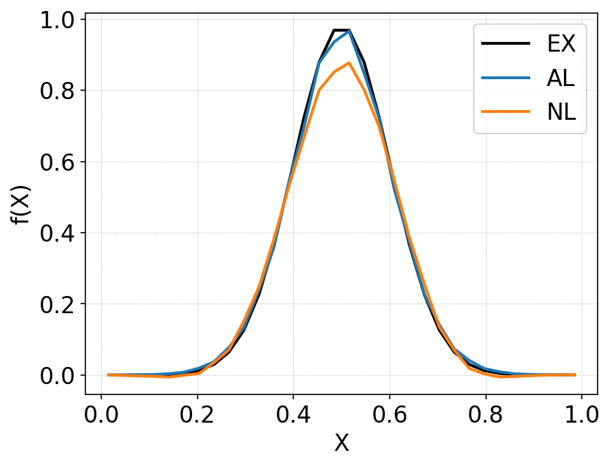
Comparison of distribution function along \(y=1/2\) between standard DG (orange line) and anti-limiter based DG (blue line). The initial condition is shown in black. Due to the anti-diffusive property of the AL-DG, the solution matches exact results more closely. The AL-DG scheme maintains positivity of cell averages as well as at control points. Small negative errors are seen in the standard DG scheme even for this smooth initial condition. See plot below.
To test if the schemes preserve positivity of cell averages, we compute
where \(N_0\) is the total number of particles in the domain at \(t=0\). This should remain constant if the scheme conserves positivity of cell averages. The figure below shows that even for this smooth initial condition, the standard DG scheme creates small amount of regions with negative cell averages.
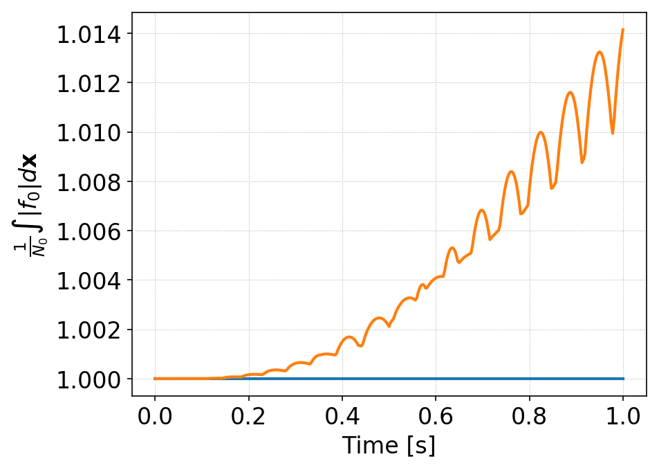
Time history of \(\int f_0 d\mathbf{x}\) for standard DG (orange) and AL-DG (blue). The AL-DG scheme preserves positivity of the cell averages exactly. In addition, though not obvious from this plot, the solution is also positive at interior control nodes.
Cylinder advection test
In this test, we initialize the simulation with a cylindrical initial condition, that is
A \(16\times 16\) grid is used and the simulation is till the cylinder, advecting diagonally. returns back to its initial position.
A line-out of the solutions along X is shown below.
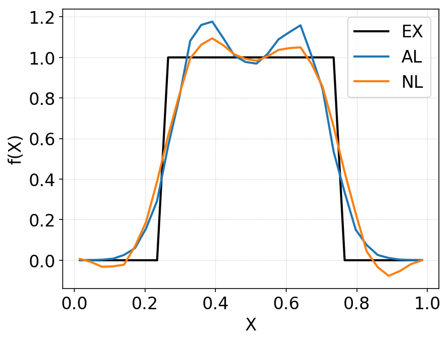
Comparison of distribution function along \(y=1/2\) between standard DG (orange line) and anti-limiter based DG (blue line), for cylindrical initial condition. The initial condition is shown in black. The standard DG scheme shows severe positivity errors, while the AL-DG scheme maintains positivity of cell-averages exactly. Due to the anti-diffusive property of the AL-DG, the monotonicity of the solution is violated more than in the standard DG scheme.
The degree with which the schemes violate positivity of cell averages is shown below:
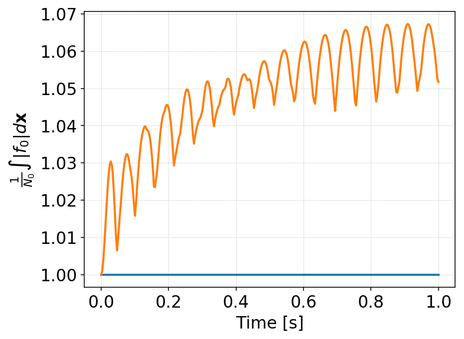
Time history of \(\int f_0 d\mathbf{x}\) for standard DG (orange) and AL-DG (blue), for cylindrical initial condition. The AL-DG scheme preserves positivity of the cell averages exactly. Note that for this case the AL-DG scheme does not enforce positivity at interior control nodes.
For this initial condition even the AL-DG scheme does not maintain positivity at interior control points. To check the impact of this, we re-run both the standard DG and AL-DG schemes with sub-cell diffusion applied as post-processing after each RK stage. To measure the amount of change we compute the following metric
where \(f^*\) is the sub-cell diffusion corrected distribution function.
The time-history of total modifications of the distribution function as well as the number of cells changed per time-step for the two schemes are shown below. Note that the anti-diffusion is applied per RK-stage.
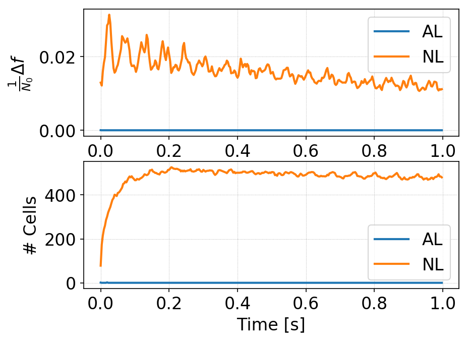
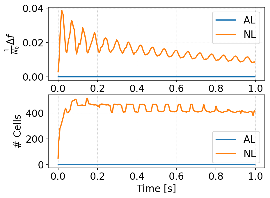
Cylindrical initial conditions. Time history of \(\Delta f\) (top) for standard DG (orange) and AL-DG (blue) and of the total number of cells changed per-step (bottom) for standard DG (orange) and AL-DG (blue). The standard DG scheme needs constant correction to about 65% of the cells in each RK stage, while the AL-DG scheme needs no corrections at all.
Square-top-hat advection test
As a severe test of the algorithm we initialize the simulation with a “square top-hat”, i.e.
A \(16\times 16\) grid is used and the simulation is till the cylinder, advecting diagonally. returns back to its initial position.
The figure below shows the final solutions computed with standard DG and AL-DG for this IC. The regions that are negative are masked out and appear as white patches.
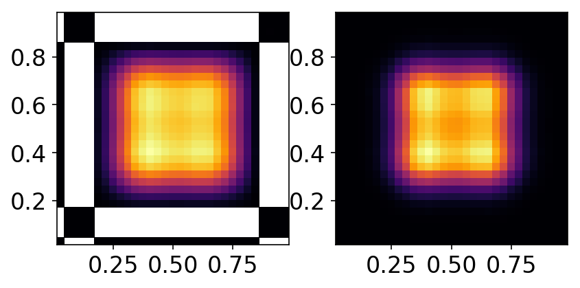
Comparison of distribution function for square-top-hat initial conditions with standard DG (left) and AL-DG (right). Regions where the distribution function goes negative are masked out and appear as white patches. Note the huge regions in which the standard DG shows positivity violation. As is also seen below, at this time in the simulation the AL-DG has no regions where the distribution function is negative.
A line-out of the solutions along X is shown below.
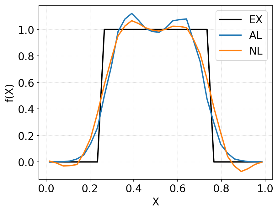
Comparison of distribution function along \(y=1/2\) between standard DG (orange line) and anti-limiter based DG (blue line), for square-top-hat initial condition. The initial condition is shown in black. The standard DG scheme shows severe positivity errors, while the AL-DG scheme maintains positivity of cell-averages exactly. Due to the anti-diffusive property of the AL-DG, the monotonicity of the solution is violated more than in the standard DG scheme.
The degree with which the schemes violate positivity of cell averages is shown below:
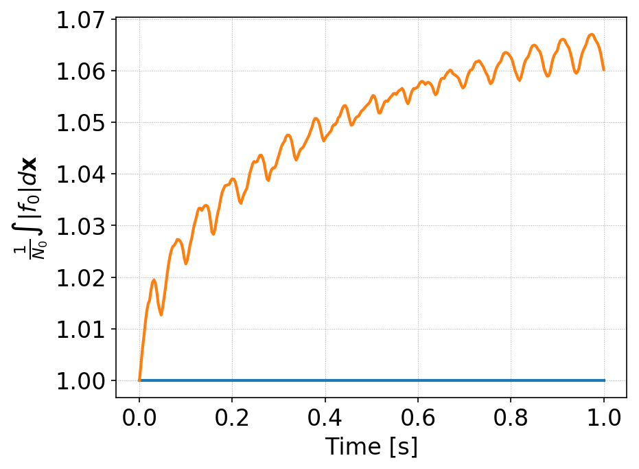
Time history of \(\int f_0 d\mathbf{x}\) for standard DG (orange) and AL-DG (blue), for square-top-hat initial condition. The AL-DG scheme preserves positivity of the cell averages exactly. Note that for this case the AL-DG scheme does not enforce positivity at interior control nodes.
For this initial condition even the AL-DG scheme does not maintain positivity at interior control points. To check the impact of this, we re-run both the standard DG and AL-DG schemes with sub-cell diffusion applied as post-processing after each RK stage.
The time-history of total modifications of the distribution function as well as the number of cells changed per time-step for the two schemes are shown below. Note that the anti-diffusion is applied per RK-stage.
Square-top-hat initial conditions. Time history of \(\Delta f\) (top) for standard DG (orange) and AL-DG (blue) and of the total number of cells changed per-step (bottom) for standard DG (orange) and AL-DG (blue). The standard DG scheme needs constant correction to about 65% of the cells in each RK stage, while the AL-DG scheme needs no corrections.
Conclusions
We have presented an anti-limiter scheme based discontinuous Galerkin scheme to handle the problem of positivity in kinetic equations. These AL-DG will conserve energy much better, perhaps even exactly (in the continuous time-limit) with additional fixes to the volume terms.
References
- Zhang2011
X. Zhang and C.W Shu. (2011). “Maximum-principle-satisfying and positivity-preserving high-order schemes for conservation laws: survey and new developments”, Proceedings of the Royal Society a: Mathematical, Physical and Engineering Sciences, 467 (2134), 2752–2776. http://doi.org/10.1098/rspa.2011.0153