JE33: “Ghost Currents” and Kinetic simulations of the Buneman Instability

Contents

• JE33: “Ghost Currents” and Kinetic simulations of the Buneman Instability

  • Ghost Currents

  • The linear stage

  • The nonlinear stage

    • Mass ratio \(m_i/m_e = 25\)

    • Mass ratio \(m_i/m_e = 1836.2\)

  • The nonlinear stage with weak collisions

  • Conclusion

  • Footnotes

In this note I study the Buneman instability with the Vlasov-Maxwell solver in Gkeyll. This is in preparation for a more complex case in which a magnetic field is also present. In the latter case the instability is called “Electron Cyclotron Drift Instability” (ECDI), often conjectured as causing anomalous electron transport observed in Hall-thrusters.

Ghost Currents

In an electrostatic (ES) problem if one uses Poisson equation as the field equation, currents do not directly appear anywhere. However, if one uses Maxwell equations (Ampere’s law) instead, the field equation becomes

\[\mu_0\epsilon_0 \frac{\partial E}{\partial t} = -\mu_0 J.\]

Hence, an initial plasma current will give rise to an electric field, that in turn drives plasma currents that tend to cancel those applied initially. An oscillation at the plasma frequency will be set up. This does not happen when using Poisson equation, however, as the currents never appear in the field equation.

This is a manifestation of the fact a current flow will result in a magnetic field that balances it. However, this effect is missing in the ES approximation. Hence, when using Ampere’s law to compute the field, we must mock up the effect of the missing magnetic field that will support a steady current.

There is another way to illustrate the difference between Poisson and Ampere’s law for fields in the electrostatic case. As \(E=-\partial\phi / \partial x\), integrating this over the domain and assuming periodic boundary conditions we get

\[\int_0^L E \ dx = \phi(0)-\phi(L) = 0\]

due to periodicity. Hence, integrating Ampere’s equation over the domain we should have

\[\mu_0\epsilon_0 \int_0^L \frac{\partial E}{\partial t} \ dx = 0 = -\mu_0 \int_0^L J \ dx\]

Obviously, this condition is impossible to satisfy if we have a net non-zero current!

In addition, if we use the electric field to compute the potential as

\[\phi(x) = \int_0^x E(x')\ dx'\]

the resulting potential will not be periodic, even if the field and distribution functions are periodic.

Hence, when using the Vlasov-Maxwell system (as opposed to the Vlasov-Poisson system) one needs some care to ensure that the ES physics is captured correctly.

One way around this is to introduce a “ghost current” that exactly cancels the plasma current. That is, we replace Ampere’s law with

\[\mu_0\epsilon_0 \frac{\partial E}{\partial t} = -\mu_0 (J+J_g).\]

Here \(J_g\) is a spatially uniform ghost current that is computed at each time step as

\[J_g = -\frac{1}{L} \int_0^L J \ dx.\]

With this choice, the right hand side of the field equation will vanish, satisfying the condition for periodicity of the potential.

Note that in general, Ampere’s law alone can’t be used to do a ES problem in more than one dimension. To see this, as \(E = -\nabla\phi\), taking the curl of Ampere’s law we get

\[\mu_0\epsilon_0 \nabla\times \frac{\partial \mathbf{E}}{\partial t} = 0 = -\mu_0 \nabla \times \mathbf{J}.\]

Obviously, there is no reason why this condition should be satisfied. Again, this is a manifestation of the fact that in the ES approximation currents do not cause magnetic fields. One can imagine adding in a ghost-current in this case also:

\[\nabla \times (\mathbf{J} + \mathbf{J}_g) = 0.\]

However, the expression to compute \(\mathbf{J}_g\) will be non-local (requiring a Poisson solve of some sort), defeating the purpose of using Ampere’s law (to exploit its locality, that is).

A more abstract explanation is as follows. As the Maxwell equations are hyperbolic while Poisson equation is elliptic, there is no way that they will give the same physics in a time-dependent situation. The above arguments about ghost currents, in fact, is a way to restore the non-locality inherent in the elliptic Poisson equation into Ampere’s law to allow one to do consistent ES simulations 1.

The linear stage

Consider a one-dimensional collisionless plasma in which the electrons are drifting with respect to cold ions with speed \(V_0\) much larger than the electron thermal speed, i.e. \(V_0 \gg v_{the}\). In this case an electron perturbation couples to ion plasma oscillations, leading to an electrostatic instability called the Buneman instability. Assuming cold ions and kinetic electrons the dispersion relation for this instability is

\[1 - \frac{\omega_{pe}^2}{2 v_{the}^2k^2} Z'\left( \frac{\omega-kV_0}{\sqrt{2}v_{the}k} \right) - \frac{\omega_{pi}^2}{\omega^2} = 0.\]

To a good approximation one can also assume that the electrons are a cold fluid. In this case the dispersion relation becomes

\[1 - \frac{\omega_{pe}^2}{(\omega-k V_0)^2} - \frac{\omega_{pi}^2}{\omega^2} = 0.\]

The solution to this dispersion relation gives good insight into the nature of the instability. Rearranging this expression, one finds that the normalized growth rate, \(\omega/\omega_{pe}\), depends only on the parameters \(k V_0/\omega_{pe}\) and \(m_e/m_i\). This dispersion relation can be solved in a couple of lines of Python (code courtesy of Liang Wang)

import numpy as np

def buneman_k2w_cold(k, m):
    """
    Args:
        k: k*v0/wpe
        m: mi/me

    Returns:
        ws: Complex frequency for the given k.
    """
    ws = np.roots((m, -2 * k * m, k**2 * m - (m + 1), 2 * k,  -k**2))
    return ws[np.argsort(ws.imag + 1j * ws.real)[::-1]]

The following plot shows the growth rate for various \(k V_0/\omega_{pe}\) as a function of mass ratio. Clearly, as expected, for a given mass-ratio the growth rate is maximized around the resonant case \(kV_0 = \omega_{pe}\).

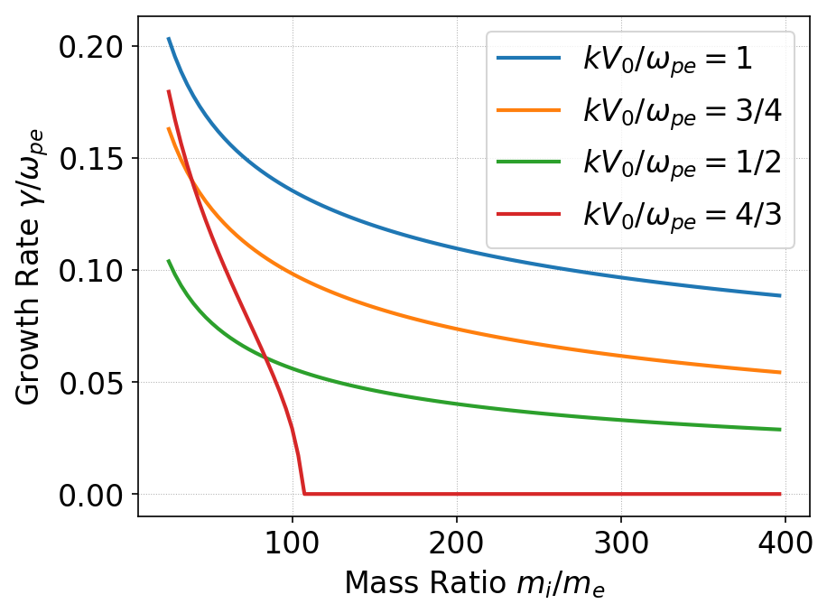
Comparison of linear growth rate for Buneman instability as function of mass ratios computed for various values of \(k V_0/\omega_{pe}\). The growth is maximum for the resonant case \(kV_0 = \omega_{pe}\). For \(kV_0/\omega_{pe} > 1\) and large enough mass-ratio there are no unstable modes, at least as predicted in the cold-fluid theory.

The following plot shows the growth rate as a function of wave-number for various mass ratios. As seen below, consistent as the above plot, the Buneman instability growth reduces with mass ratio and beyond a certain wave-number the growth is zero.

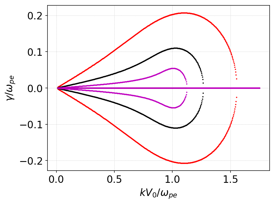
Growth rate for Buneman instability as function of wave-number for various values of mass ratios: red \(m_i/m_e = 25\), black \(m_i/m_e = 200\) and magenta \(m_i/m_e = 1836.2\). Growth reduces with mass ratio and beyond a certain wave-number becomes zero.

The Buneman instability also has a oscillatory component as seen in the following plot. It shows the growth rate as a function of oscillation frequency for different mass ratios.

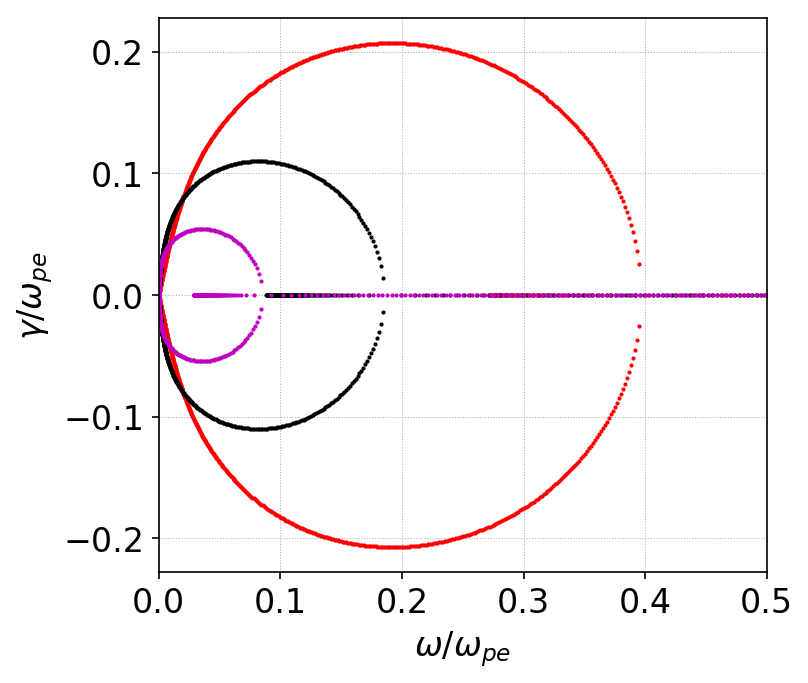
Growth rate for Buneman instability as function of oscillation frequency for various values of mass ratios: red \(m_i/m_e = 25\), black \(m_i/m_e = 200\) and magenta \(m_i/m_e = 1836.2\). Consistent with the previous figures, purely oscillatory modes exist beyond a critical oscillation frequency.

As seen in the above plots, the maximum growth of the instability occurs approximately at resonance \(kV_0 = \omega_{pe}\). In this resonant case, as \(V_0 \gg v_{the}\), we have \(\omega_{pe} \gg k v_{the}\). One can then show that the growth rate can be approximately computed as

\[\frac{\gamma}{\omega_{pe}} = \frac{\sqrt{3}}{2} \left( \frac{m_e}{2m_i} \right)^{1/3} \left[ 1 - \frac{1}{2} \left( \frac{m_e}{2m_i} \right)^{1/3} \right].\]

In the first series of tests I initialized a simulation with stationary ions with \(v_{the} = 1/50\), \(v_{thi}=10^{-3}\) and drift speed determined from resonance condition \(V_0 = \omega_{pe}/k\). Mass ratio \(m_i/m_e\) of \(25, 50, 100, 200, 400, 1836.2\) and \(40\times 1836.2\) (Argon ions) were used. The linear growth rate was computed using the Postgkyl “growth” command and results compared to values computed from the above formula. The results are shown in the figure below. The agreement with analytical theory is very good, giving confidence in the numerical solutions. (For an exact comparison one would need to solve the full kinetic dispersion relation, something I have not yet done).

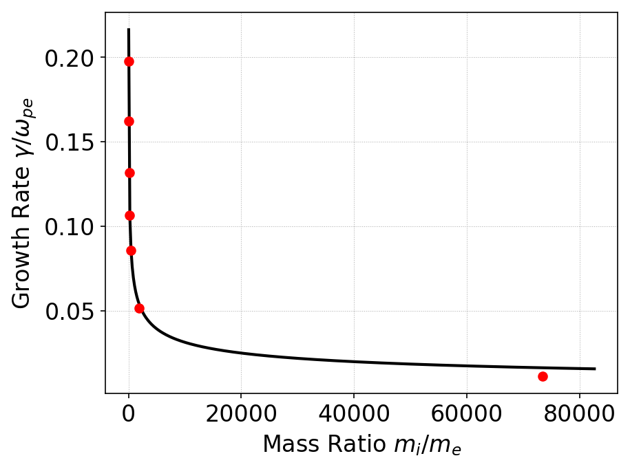
Comparison of linear growth rate for Buneman instability with various mass ratios computed from Gkeyll simulations (red dots) and analytical formula given in text (black). The growth rate of the instability reduces rapidly with increasing ion mass (approximately \((m_e/m_i)^{1/3}\)). Note that this is for the resonant case in which \(k V_0 = \omega_{pe}\). See es-buneman/b1, es-buneman/b2, es-buneman/b3, es-buneman/b4, es-buneman/b5, es-buneman/b6, es-buneman/b7 for input files.

The nonlinear stage

After a few multiples of \(\tau = 1/\gamma\), the linear growth stops and the instability saturates. This saturation is due to the slowing down of the electrons in the increasing electric field and mode coupling to the ions. The electric field increases sufficiently that some electrons no longer have the energy to cross the potential barrier, and this eventually leads to particle trapping. As the trapping continues the electron distribution flattens, moving the system into a quasi-steady state.

Mass ratio \(m_i/m_e = 25\)

I looked at two non-linear cases, the first with \(m_i/m_e = 25\), and the other for a hydrogen plasma, i.e. \(m_i/m_e = 1836.2\). The field energy as a function of time is plotted below for the \(m_i/m_e = 25\) case.

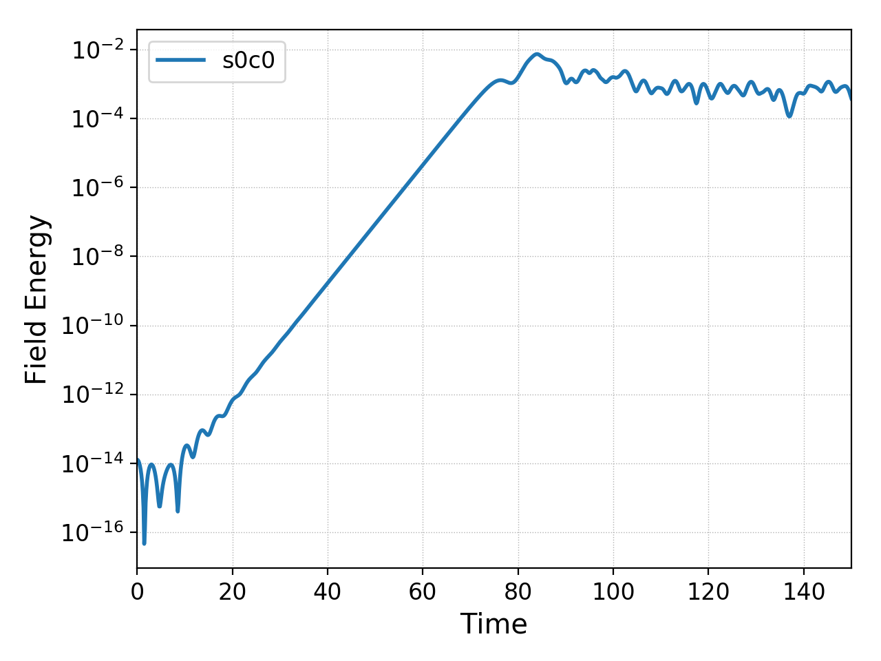
Field energy for \(m_i/m_e = 25\) case as a function of time. The growth period for this case is \(\tau = 1/\gamma \approx 5\). The instability saturates about \(t\omega_{pe} = 70\), followed by a second growth phase and then saturation. See es-buneman/n1 for input file.

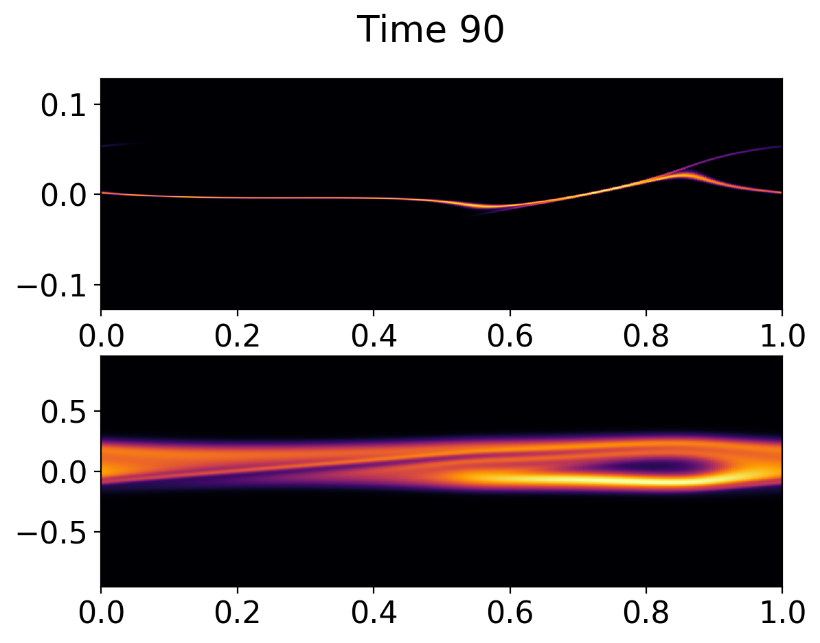
The plot below shows the ion (top) and electron (bottom) distribution at \(t\omega_{pe} = 90\). At this point electrons are trapped in the electrostatic field.

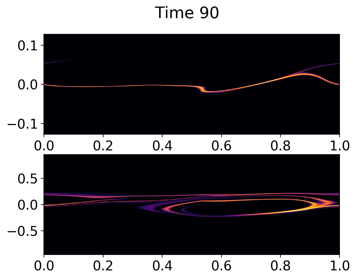
Ion (top) and electron (bottom) distribution function at \(t\omega_{pe} = 90\). The electrons distribution function shows particle trapping which leads to the slowing down of the electron bulk velocity. As the ions are not very heavy they show significant acceleration in the field.

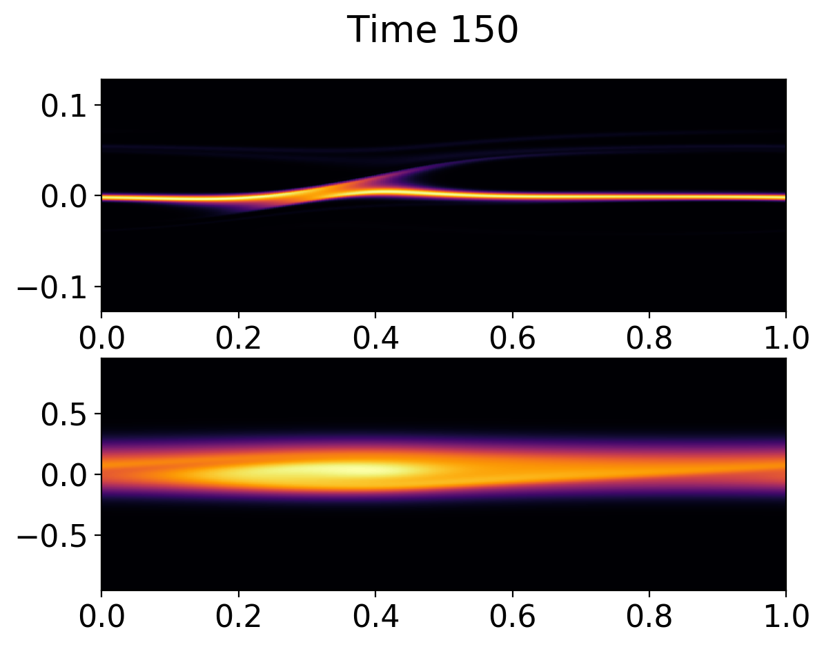
Deep in the nonlinear phase the electron trapping leads to a flattening of the distribution function, showing complex fine-scale features in the trapped region. However, a fraction of passing particles are also present. See below.

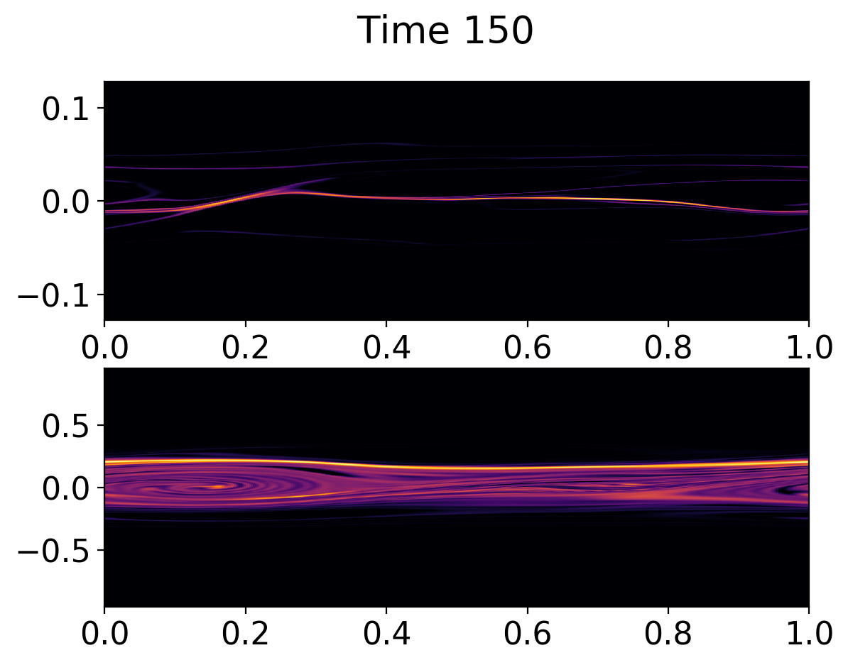
Ion (top) and electron (bottom) distribution function at \(t\omega_{pe} = 150\). In this deeply nonlinear phase of the instability the electron distribution had flattened due to the particle trapping. However, a significant fraction of passing particles are also present.

Mass ratio \(m_i/m_e = 1836.2\)

For hydrogen ions the growth is slower and the particle trapping leads to significant flattening of the distribution function. The following plot shows the field energy as a function of time.

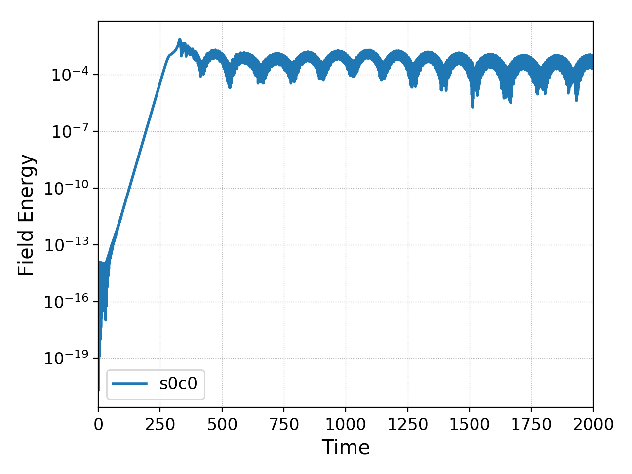
Field energy for \(m_i/m_e = 1836.2\) case as a function of time. The instability saturates about \(t\omega_{pe} = 250\), followed by a second growth phase and then saturation. After saturation there is a periodic exchange of energy between the electric field and ions. See es-buneman/n6 for input file.

Around \(t\Omega_{pe} = 320\) particle trapping is significant, as seen in the plot below.

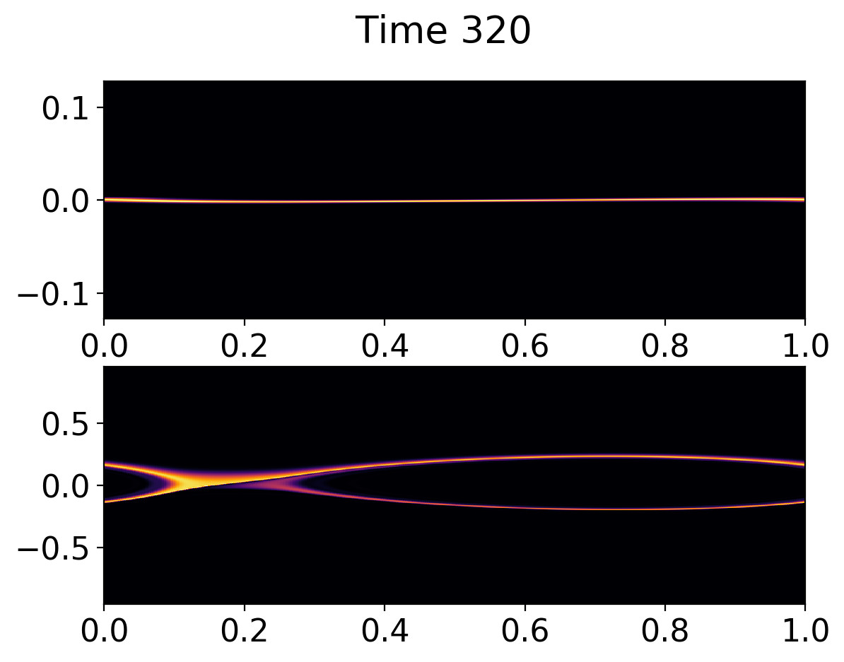
Ion (top) and electron (bottom) distribution function at \(t\omega_{pe} = 320\). The electrons distribution function shows particle trapping which leads to the slowing down of the electron bulk velocity.

Deep in the nonlinear phase particle trapping leads to flattening of the distribution function, though a persistent electron hole seems to be present. Some fraction of passing particles are also seen.

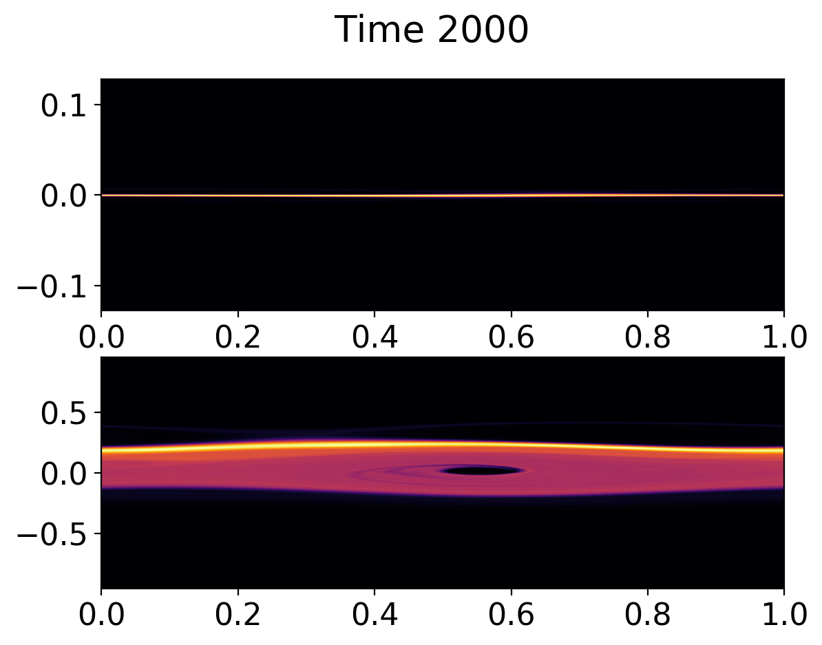
Ion (top) and electron (bottom) distribution function at \(t\omega_{pe} = 2000\). The electrons distribution function has flattened due to particle trapping, although a persistent electron hole seems to be present. Small fraction of passing particles are also present.

The flattening is better seen in the following plot that shows \(\int_0^L f(x,v,t)\ dx\) at \(t\omega_{pe}=0\) and \(t\omega_{pe}=2000\). A small fraction of passing particles are clearly visible.

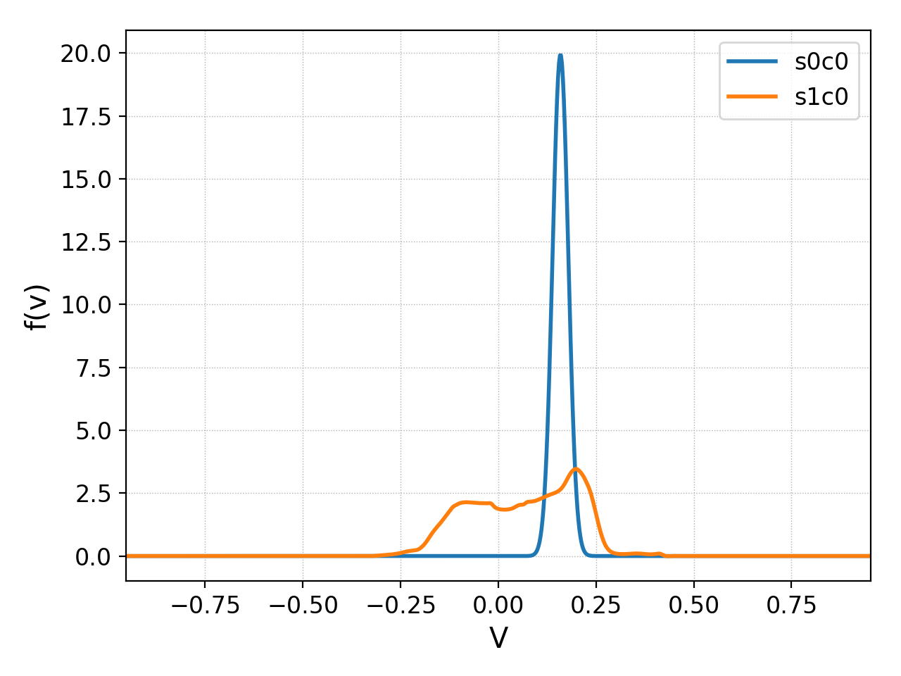
Spatially integrated distribution function at \(t\omega_{pe}=0\) (blue) and \(t\omega_{pe}=2000\). Flattening due to trapping is clearly visible. A small fraction of passing particles are also seen.

The nonlinear stage with weak collisions

The final set of simulations I performed were included weak electron-electron collisions for the \(m_i/,_e = 25\) case. For this the collision frequency was set to \(\nu_{ee}/\omega_{pe} = 10^{-2}\) and a Lenard-Bernstein Operator (LBO) was used. This operator conserves density, momentum and energy and has the same structure as the full Fokker-Planck operator in that it has a drag and diffusion term. However, it does not require the calculation of Rosenbluth potentials, which, even though it simplified the implementation, implies that it can not capture the correct velocity dependent collision frequency.

The collisions are sufficiently weak that the linear phase of the instability is unchanged. See field energy plot below.

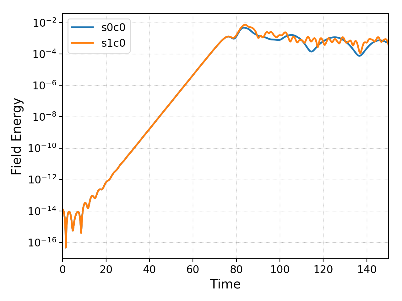
Field energy for \(m_i/m_e = 25\) case as a function of time. Blue curve shows the case with weak collisions (\(\nu_{ee}/\omega_{pe}=10^{-2}\)) and the orange line is the collisionless case. The linear phase of the instability is unchanged with collisions, but the small-scale field energy oscillations are wiped out. See es-buneman/c1 for input file.

However, the non-linear phase is qualitatively different, with most of the fine-scale phase-space structures wiped out due to collisions. However, qualitative features like particle trapping and flattening of distribution function persist. The following plots show the distribution functions at \(t\omega_{pe} = 90\) and \(t\omega_{pe} =150\). These should be compared with the collisionless case above.

Ion (top) and electron (bottom) distribution function at \(t\omega_{pe} = 90\) with weak collisions. The fine-scale features in the collisionless case are wiped out, even with weak collisions.

Same as previous figure, except at \(t\omega_{pe} = 150\).

The following plot shows the spatially integrated distribution function at \(t\omega_{pe} = 100\) for the collisionless and collisional cases. Note that the finer phase-space features are wiped out and the distribution function is becoming Maxwellian due to the collisions. By \(t\omega_{pe}=150\) the collisions cause near thermalization of the electrons.

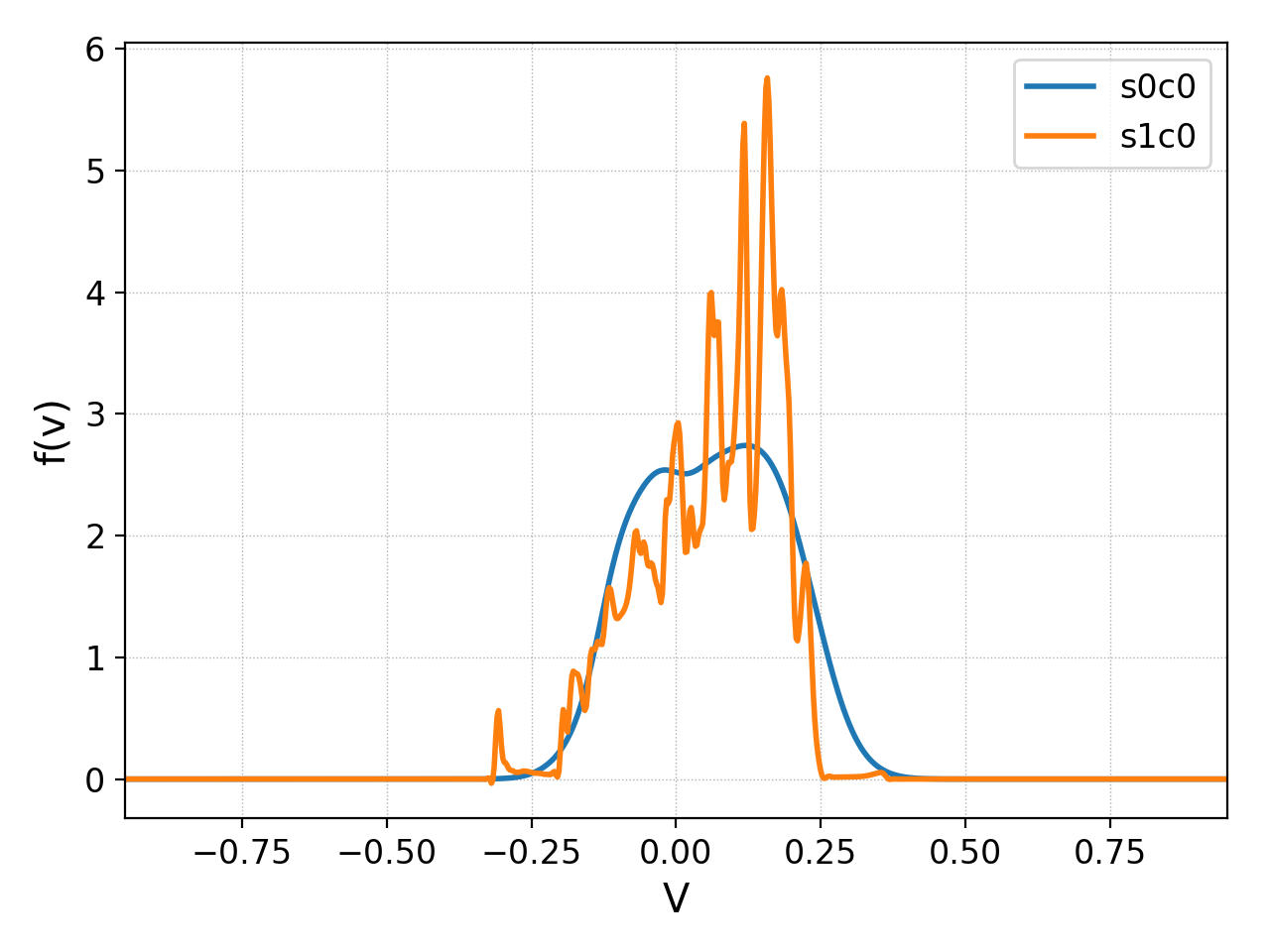
Spatially Integrated distribution function; blue curve shows the case with weak collisions (\(\nu_{ee}/\omega_{pe}=10^{-2}\)) and the orange line is the collisionless case. The collisions wipe out the fine-scale distribution function features and drive the electrons towards thermalization. However, at this point some flattening continues to persist.

Conclusion

Simulations of Buneman instability (or any electrostatic problems) with a Vlasov-Maxwell code are tricky. Non-locality needs to be introduced via ghost currents and, in general, multidimensional electrostatic simulations are not possible with just Ampere’s law. One would need to solve Poisson equation as the non-locality is inescapable.

Many interesting features are seen in the simulations, including saturation due to particle trapping, complex phase-space structures and highly persistent electron holes. Even weak collisions can have a significant quantitative impact in the late nonlinear phase of the instability. This study sets the path to perform simulations with magnetized electrons, a case relevant to potentially explain anomalous electron transport in Hall thrusters and other \(E\times B\) machines.

Footnotes

1

I am grateful to Greg Hammett for discussion on aspects of performing ES simulations with Maxwell equations.