JE19: On diffusion operators with discontinuous Galerkin schemes

Contents

• JE19: On diffusion operators with discontinuous Galerkin schemes

  • Implementation notes

  • Convergence of recovery DG scheme in 1D

  • Convergence of recovery DG scheme in 2D

  • References

In this note I describe and test a DG scheme for solving the diffusion equation using the recovery procedure proposed by van Leer [vanLeer2005].

Consider the problem of computing the second derivative of a function

\[g = f_{xx}\]

where \(f(x)\) is some function. As the DG representation of \(f(x)\) is, in general, discontinuous across cell boundaries it is not clear how to compute \(g(x)\). Multiply the equation by a test function \(\varphi(x)\) and integrate over a cell \(I_j \equiv [x_{j-1/2},x_{j+1/2}]\) to get

\[\int_{I_j} \varphi g dx = (\varphi f_x - \varphi_x f)\bigg|^{x_{j+1/2}}_{x_{j-1/2}} + \int_{I_j} \varphi_{xx} f dx\]

where integration by parts had been used twice. Note that as the function \(f(x)\) is discontinuous across cell edges, it is not clear how to evaluate the terms inside the bracket in the above weak-form.

The recovery discontinuous Galerkin (RDG) scheme proposed by van Leer replaces the the function \(f(x)\) at each edge by a recovered polynomial that is continuous across the cells shared by that edge. I.e., we write instead the weak form

\[\int_{I_J} \varphi g dx = (\varphi \hat{f}_x - \varphi_x \hat{f})\bigg|^{x_{j+1/2}}_{x_{j-1/2}} + \int_{i_J} \varphi_{xx} f dx\]

where \(\hat{f}(x)\) is the recovered polynomial, continuous across a cell edge. As the recovered polynomial is continuous, its derivative can be computed and used in the above weak-form, allowing us to compute \(g(x)\).

Consider an edge \(x_{j-1/2}\). To recover a polynomial that is continuous in cells \(I_{j-1}\) and \(I_{j}\) that share this edge, we use \(L_2\) minimization to give the conditions

\[\begin{split}\int_{I_{j-1}} (\hat{f}-f) \varphi_{j-1} dx &= 0 \\ \int_{I_{j}} (\hat{f}-f) \varphi_{j} dx &= 0\end{split}\]

This ensures that \(\hat{f}\), defined over \(I_{j-1}\cup I_j\) is identical to \(f(x)\) in the least-square sense.

The reconstruction procedure is more complicated in higher dimensions, specially when using non-rectangular meshes. For now, we have developed a systematic method of computing the recovery polynomial for arbitrary basis on rectangular meshes and this has been implemented in Gkeyll. This will be extended to general non-rectangular meshes in the future.

Implementation notes

The NodalHyperDiffusionUpdater implements the diffusion operator and computes (in 1D)

\[g = f + \Delta t \nu f_{xx}\]

or, if the incrementOnly flag is specified,

\[g = \nu f_{xx}\]

where, \(f(x,t)\) is the input field, \(g(x,t)\) is the output field, \(\nu\) is a diffusion coefficient and \(\Delta t\) is the time-step. Multiple calls to the updater can then be combined in a RK time-stepper to solve a diffusion equation, for example.

Convergence of recovery DG scheme in 1D

To test the convergence of the scheme a series of 1D simulations were performed. The heat-conduction equation was solved on a domain \([0,2\pi]\) with diffusion coefficient \(1.0\). The initial condition was a single mode \(\sin(x)\). The exact solution for this problem is \(e^{-t}\sin(x)\).

The time-step was held fixed while 8, 16, 32, and 64 cell grids were used. The results are shown in the following tables for polynomial order 1 and 2 nodal basis functions.

Note

To compute these errors I am compared the solution to exact solution at \(t=1\). The convergence rates are lower than what I expected from linear analysis. However, this could be due to the way in which the errors are computed. I plan to fix this later.

Convergence of polynomial order 1 recovery DG scheme

Grid size \(\Delta x\)	Average error	Order	Simulation
\(2\pi/8\)	\(3.54322\times 10^{-3}\)		s242
\(2\pi/16\)	\(4.64979\times 10^{-4}\)	2.92	s243
\(2\pi/32\)	\(5.88495\times 10^{-5}\)	2.98	s244
\(2\pi/64\)	\(7.37923\times 10^{-6}\)	2.99	s245

---

Convergence of polynomial order 2 recovery DG scheme

Grid size \(\Delta x\)	Average error	Order	Simulation
\(2\pi/4\)	\(8.101\times 10^{-3}\)		s246
\(2\pi/8\)	\(9.600\times 10^{-4}\)	3.0	s247
\(2\pi/16\)	\(1.186\times 10^{-4}\)	3.0	s248
\(2\pi/32\)	\(1.479\times 10^{-5}\)	3.0	s249

Convergence of recovery DG scheme in 2D

To test the convergence of the scheme a series of 2D simulations were performed. The heat-conduction equation was solved on a domain \([0,2\pi]\times[0,2\pi]\) with diffusion coefficient \(1.0\). The initial condition was \(\sin(x)\cos(y)\). The exact solution for this problem is \(e^{-2t}\sin(x)\cos(y)\).

The time-step was held fixed while grid sizes of \(8\times 8\), \(16\times 16\), \(32\times 32\) and \(64\times 64\), cell grids were used. The following figure shows the results from the \(16\times 16\) case compared to the exact solution.

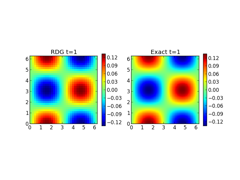
Solution to diffusion equation in 2D with recovery DG scheme (left) and exact solution (right). The simulation [s251] was run on a \(16\times 16\) grid.

References

vanLeer2005

van Leer, Bram and Nomura, Shohei, “Discontinuous Galerkin for Diffusion”, 17th AIAA Computational Fluid Dynamics Conference, AIAA 2005-5108.