JE1: Solving Poisson equation on 2D periodic domain

The problem and solution technique

With periodic boundary conditions, the Poisson equation in 2D

(1)\[\frac{\partial^2 \psi}{\partial x^2} + \frac{\partial^2 \psi}{\partial y^2} = s(x,y)\]

can be solved using discrete Fourier transforms. Denote the rectangular domain by \(\Omega\) and discretize using \(N_x \times N_y\) cells.

Integrating (1) over \(\Omega\) and using periodicity shows that the source \(s(x,y)\) must satisfy

\[\int_\Omega s(x,y) dx dy = 0\]

In the solver implemented in Lucee the source is modified by subtracting the integrated source from the RHS of (1) to ensure that this condition is met. Hence, the solution computed by the updater does not satisify (1) but the modified equation

(2)\[\frac{\partial^2 \psi}{\partial x^2} + \frac{\partial^2 \psi}{\partial y^2} = s(x,y) - s_T\]

where \(s_T = \int_\Omega s(x,y) dx dy / |\Omega|\), where \(|\Omega|\) is the domain volume. Note that for a properly posed problem the zero integrated source condition must be met.

Once the source term is adjusted, its 2D Fourier transform is computed. The Fourier transform of the solution is then

\[\overline{\psi}(k_x, k_y) = -\frac{\overline{s}(k_x,k_y)}{k_x^2+k_y^2}\]

where overbars indicate 2D Fourier transforms and \(k_x\) and \(k_y\) are the wave-numbers. The zero wave-numbers are replaced by \(10^{-8}\) to prevent divide-by-zero. The FFTW library is used to compute the transforms.

The algorithm is implemented in the class PeriodicPoisson2DUpdater class in the proto directory.

This updater is for use in testing finite-volume/finite-difference 2D incompressible flow algorithms. In this entry the stand-alone updater is verified.

Test Problem 1

The domain is assumed to be \(\Omega = [-L_x/2, L_x/2] \times [-L_y/2, L_y/2]\) with \(L_x=L_y=2\) and is discretized using \(128\times 128\) cells. The source is an isotropic Gaussian source of the form

\[s(x,y) = e^{-10(x^2+y^2)}\]

The source and the numerical solution is shown below.

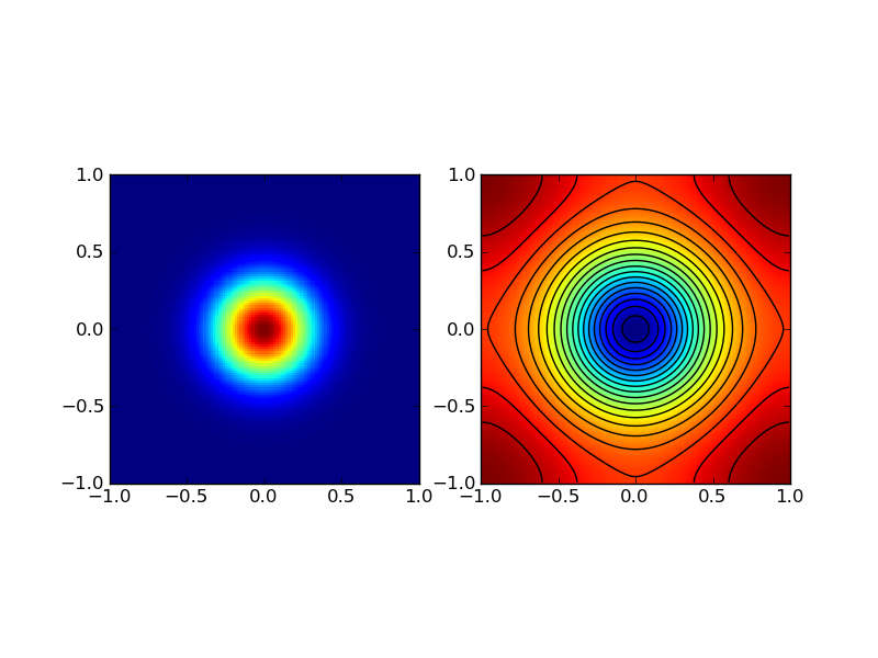
The source (left) for this problem [s1] is an isotropic Gaussian \(e^{-10(x^2+y^2)}\). Color and contour plot of the solution is shown in the right plot.

A central difference operator is applied to the computed solution and is compared to the adjusted source. The results are shown below.

Central difference of the solution (black line) compared to the source (red dots) along the X-axis (left) and Y-axis (right).

Test Problem 2

The domain and resolution are the same as problem 1. The source is an anisotropic Gaussian source of the form

\[s(x,y) = e^{-10(2x^2+4xy+5y^2)}\]

The source and the numerical solution is shown below.

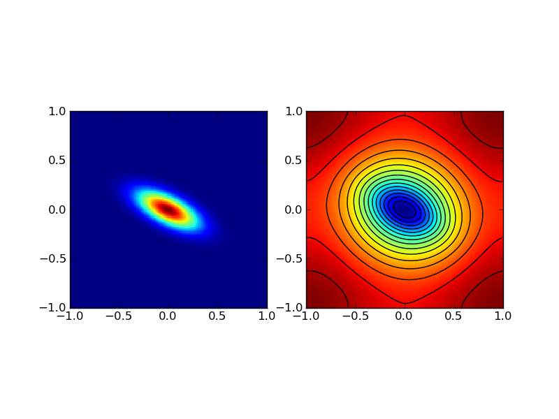
The source (left) for this problem [s2] is an anisotropic Gaussian \(e^{-10(2x^2+4xy+5y^2)}\). Color and contour plot of the solution is shown in the right plot.

A central difference operator is applied to the computed solution and is compared to the adjusted source. The results are shown below.

Central difference of the solution (black line) compared to the source (red dots) along the X-axis (left) and Y-axis (right).

Test Problem 3

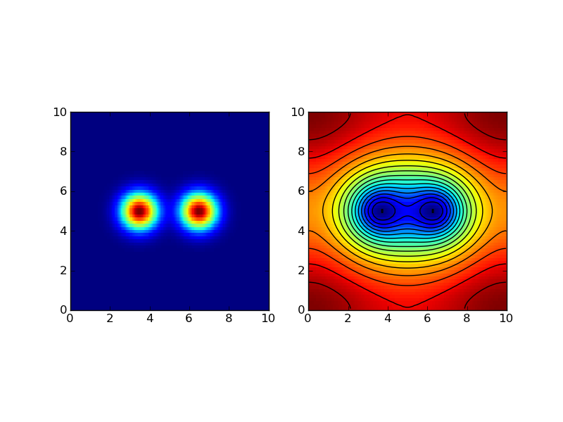
The domain is assumed to be \(\Omega = [0, L_x] \times [0, L_y]\) with \(L_x=L_y=10\) and is discretized using \(128\times 128\) cells. The source is the sum of two Gaussians given by

\[s(x,y) = \omega_1(x,y) + \omega_2(x,y)\]

where

\[\omega_i(x,y) = e^{-r_i^2/0.8}\]

where \(r_i^2 = (x-x_i)^2 + (y-y_i)^2\) and \((x_1,y_1) = (3.5,5.0)\) and \((x_2,y_2) = (6.5,5.0)\). The source and the numerical solution is shown below.

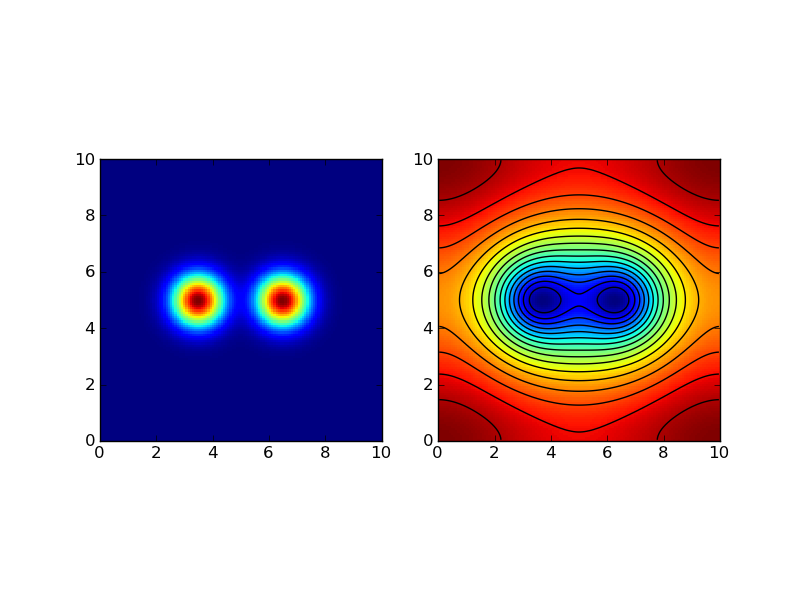
The source (left) for this problem [s3] is the sum of two Gaussians. Color and contour plot of the solution is shown in the right plot.

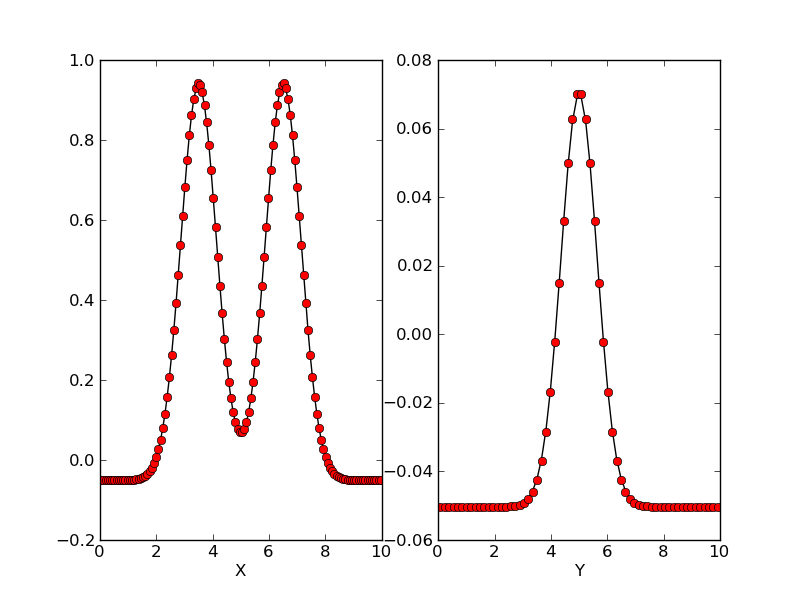
A central difference operator is applied to the computed solution and is compared to the adjusted source. The results are shown below.

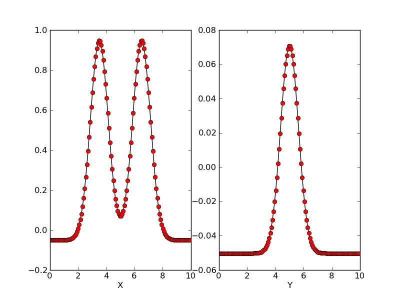
Central difference of the solution (black line) compared to the source (red dots) along the X-axis (left) and Y-axis (right).

Test Problem 4

This problem is the same as Test Problem 3 except it is discretized using \(128\times 64\) cells. The solutions are shown below.

The source (left) for this problem [s4] is the sum of two Gaussians. Color and contour plot of the solution is shown in the right plot.

A central difference operator is applied to the computed solution and is compared to the adjusted source. The results are shown below.

Central difference of the solution (black line) compared to the source (red dots) along the X-axis (left) and Y-axis (right).