JE4: Two-fluid electromagnetic Riemann problems

Contents

• JE4: Two-fluid electromagnetic Riemann problems

  • Initial conditions

  • Overview of solution procedure

  • Case 1: \(q_i/m_i = 1\)

  • Case 2: \(q_i/m_i = 10\)

  • Case 3: \(q_i/m_i = 100\)

  • Case 4: \(q_i/m_i = 1000\)

  • References

In this entry I present solutions of Riemann problems for two-fluid plasma equations. These problems are not physical but illustrate the basic mathematical structure of two-fluid solution. There are no exact solutions to these problems and reference numerical solutions are published in [Hakim2006] and [Loverich2011] using two different methods (wave-propagation and discontinuous Galerkin schemes). In this note I test the ability of the wave-propagation scheme to solve the two-fluid equations.

Initial conditions

The initial conditions are two constant states separated at \(x=0.5\). The states left and right initial states are given by

\[\begin{split}\left[ \begin{matrix} \rho_e \\ u_e \\ v_e \\ w_e \\ p_e \\ \rho_i \\ u_i \\ v_i \\ w_i \\ E_x \\ E_y \\ E_z \\ B_x \\ B_y \\ B_z \end{matrix} \right]_l = \left[ \begin{matrix} 1.0 m_e/m_i \\ 0 \\ 0 \\ 0 \\ 5\times 10^{-5} \\ 1.0 \\ 0 \\ 0 \\ 0 \\ 5\times 10^{-5} \\ 0 \\ 0 \\ 0 \\ 0.75\times 10^{-2} \\ 0.0 \\ 1.0\times 10^{-2} \end{matrix} \right] \qquad \left[ \begin{matrix} \rho_e \\ u_e \\ v_e \\ w_e \\ p_e \\ \rho_i \\ u_i \\ v_i \\ w_i \\ E_x \\ E_y \\ E_z \\ B_x \\ B_y \\ B_z \end{matrix} \right]_r = \left[ \begin{matrix} 0.125 m_e/m_i \\ 0 \\ 0 \\ 0 \\ 5\times 10^{-6} \\ 0.125 \\ 0 \\ 0 \\ 0 \\ 5\times 10^{-6} \\ 0 \\ 0 \\ 0 \\ 0.75\times 10^{-2} \\ 0.0 \\ -1.0\times 10^{-2} \end{matrix} \right]\end{split}\]

The domain is \(0<x<1\) and the simulations are run to \(t=10\). The mass ratio is set to \(m_e/m_i = 1/1836.2\). Simulations are run with with \(q_i/m_i = 1,10,100,1000\). These choices seem odd and very artificial but essentially increasing \(q_i/m_i\) reduces the ion-skin depth (relative to the domain size) and drives the plasma regime to ideal-MHD.

Overview of solution procedure

There isn’t a two-fluid solver in Lucee. The two-fluid equations can be solved by combining the electron and ion solutions (Euler equations) with the electromagnetic field solutions via source terms. Hence, the overall solution procedure is to evolve the fluids and fields independently and then couple them via source terms (Lorentz forces and current). This makes the Lua program to solve the two-fluid system a bit complicated as each of the steps needs to be programmed up separately. However, this has the advantage that different schemes can be used for each of the subsystems (fluids and/or fields) to get a more accurate and robust solution. In particular, it would be possible (and perhaps required) to use a different scheme for Maxwell equations than preserves the divergence constraints on the electric and magnetic field. This was not done in the simulations performed in this note.

Case 1: \(q_i/m_i = 1\)

In this simulation 1000 grid points were used to solve the equations. The results are shown below.

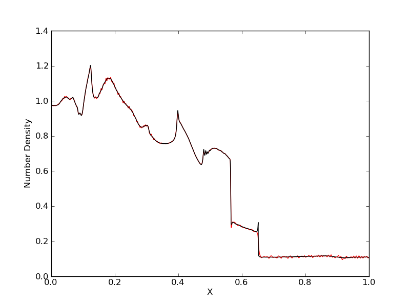
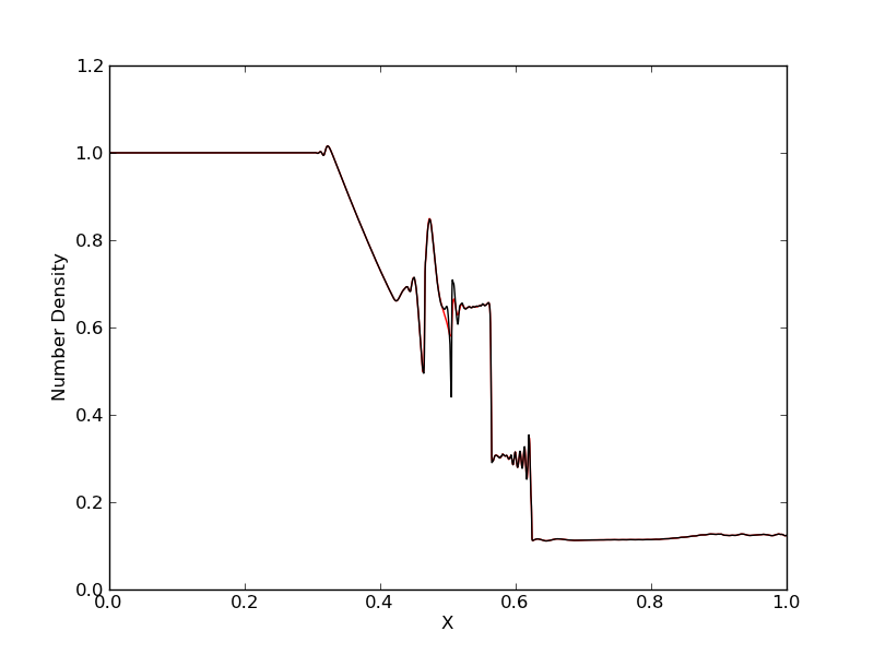
Electron number density (red) compared with ion number density (black) for simulation [s36] with \(q_i/m_i = 1\). Significant charge separation is seen.

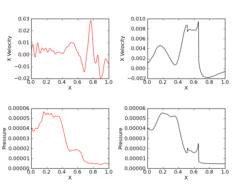
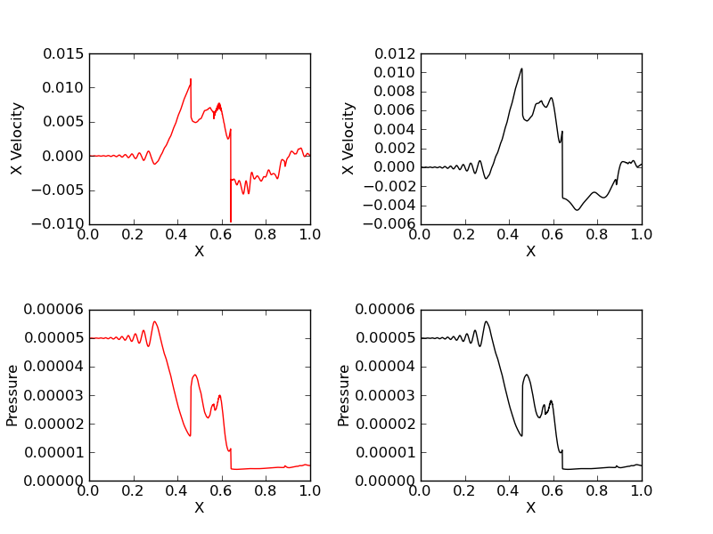
Electron (red) and ion (black) x-velocity (top row) and pressure (bottom row).

Case 2: \(q_i/m_i = 10\)

In this simulation 5000 grid points were used to solve the equations. The results are shown below.

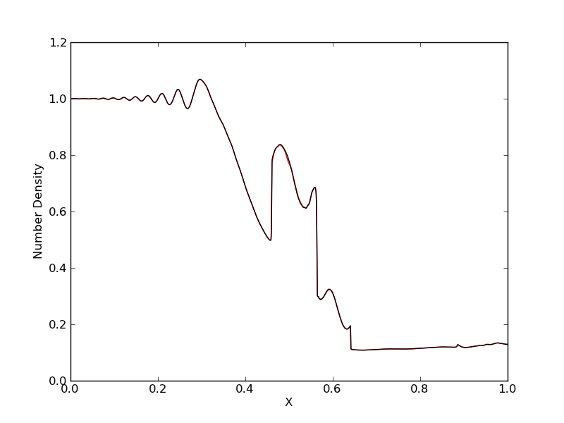
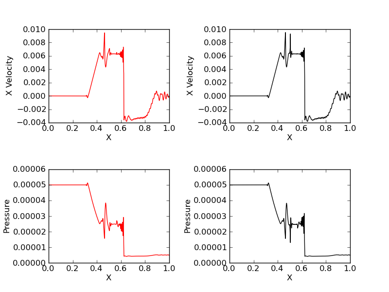
Electron number density (red) compared with ion number density (black) for simulation [s37] with \(q_i/m_i = 10\). The charge separation is seen to reduce.

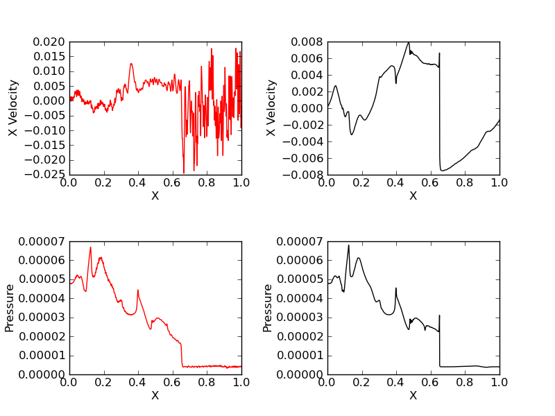
Electron (red) and ion (black) x-velocity (top row) and pressure (bottom row).

Case 3: \(q_i/m_i = 100\)

In this simulation 5000 grid points were used to solve the equations. The results are shown below.

Electron number density (red) compared with ion number density (black) for simulation [s38] with \(q_i/m_i = 100\).

Electron (red) and ion (black) x-velocity (top row) and pressure (bottom row).

Case 4: \(q_i/m_i = 1000\)

Note

The claim below that “the limiting time-step for stability is due to the plasma frequency” is no longer true in the latest version of Gkeyll, which implements a locally implicit scheme. A CFL of 1.0 can be used, leading to a 10X speedup in the simulation.

In this simulation 5000 grid points were used to solve the equations. With this charge to mass ratio the limiting time-step for stability is due to the plasma frequency. The CFL number needs to be reduced to 0.1 due to which the simulation takes a long time to run (more than 4 hours on a new Mac laptop). The results are shown below.

Electron number density (red) compared with ion number density (black) for simulation [s39] with \(q_i/m_i = 1000\).

Electron (red) and ion (black) x-velocity (top row) and pressure (bottom row).

References

Hakim2006

A. Hakim, J. Loverich, U. Shumlak, “A high resolution wave propagation scheme for ideal Two-Fluid plasma equations”, Journal of Computational Physics, 219, 2006.

Loverich2011

John Loverich, Ammar Hakim and Uri Shumlak. “A Discontinuous Galerkin Method for Ideal Two-Fluid Plasma Equations”, Communications in Computational Physics, 9 (2), Pg. 240-268, 2011.