JE32: Test distribution in an electromagnetic field: stochastic heating
Contents
In this note I study the motion of particles in a specified electromagnetic field. For certain time-dependent fields, the motion of particles can become stochastic, leading to heating of the particles. The question one can ask: what is the connection between stochastic motion and structure of distribution functions? This is not a trivial problem: even though the Vlasov equation contains all the information of single-particle motion, the connection between the two is not obvious in general situations. In this note some tests are performed for some simple situations to ensure that the basic algorithms in Gkeyll are capable of handling these types of problems.
Note that the fields are not self-consistently coupled to the particles. That is, even though the particles move in the specified fields, the currents do not modify the fields. Hence, these problems can be considered to belong to the class of “test distribution” simulations.
Uniform time-dependent electric field
In the first test the magnetic field is constant and pointing in the z-direction, \(\mathbf{B} = B_0 \mathbf{e}_z\). The electric field is time-dependent (but spatially uniform) and is given by
I only consider the motion of ions in this field. This problem is essentially a forced-harmonic oscillator. The particle velocities are described by two coupled ODEs:
where I am assuming \(q = m = B_0 = 1\). (This means that \(\omega\) is normalized to ion-cyclotron frequency and time is measured in its inverse). We can solve this system rather easily (convert to uncoupled second order ODEs and find particular solution for each) to get
where \(w_{x,y}(t)\) are given by, for non-resonant case \(\omega \neq 1\) as
For the resonant case, \(\omega =1\), these are given by
As the distribution function remains constant along characteristics, if initial distribution of the particles is given by \(f_0(v_x,v_y)\), the distribution at any time is
In general, using this formula, the exact solution of the characteristics derived above can be used to compute the distribution function at any given time. However, consider the special case of a Maxwellian
Using the solution above we can show that
which shows that the exact solution with an initial Maxwellian distribution is simply a drifting Maxwellian with drift velocity given by \(w_x(t), w_y(t)\).
Non-resonant case
In the first test I initialize a 1x2v simulation with \(\omega = 0.5\) and \(E_0 = 1.0\) on a \(2\times 16\times 16\) grid with Serendipity \(p=2\) basis functions. The simulation is run to \(t=100\).
For this case the phase-space orbits (starting at \(v_x=v_y=0.0\)) are periodic and are shown as a thin white line in the figures and movie of distribution function.
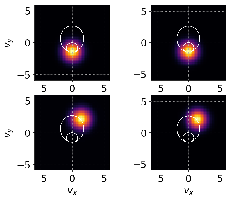
Comparison of Gkeyll distribution function (left column) and exact distribution function (right column) for test-particles in a oscillating electric (but uniform) field. Magnetic field is constant. The white line is the phase-space orbit starting at \(v_x=v_y=0.0\). The orbit is periodic and the solution is a drifting Maxwellian. This plot shows that Gkeyll solutions compares very well with the exact solution. See vlasov-test-ptcls/c2 for input file.
A more quantitative comparison can be made by plotting the drift velocities from the simulation and the exact result. This plot is shown below.
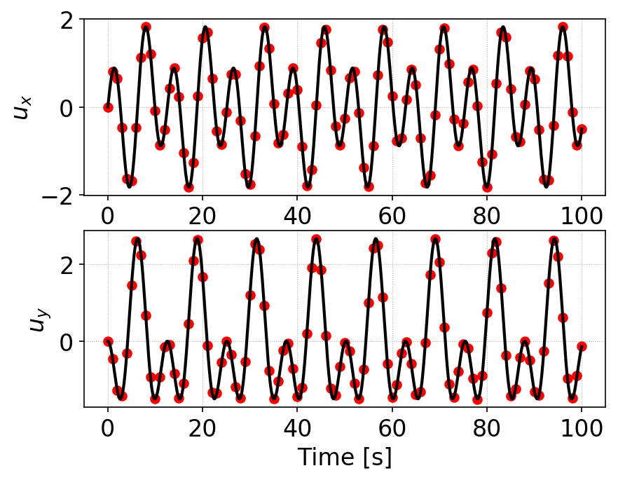
Comparison of x-component (top) and y-component (bottom) of drift velocities from simulation (red dots) with exact solution (black lines). The Gkeyll solutions compares very well with the exact solution.
Resonant case
In the test I initialize a 1x2v simulation with \(\omega = 1.0\) and \(E_0 = 0.5\) on a \(2\times 20\times 20\) grid with Serendipity \(p=2\) basis functions. The simulation is run to \(t=20\).
In the resonant case the velocity increases with time and the phase-space orbit is a spiral. Eventually the velocity increases so much that the test-particle picture breaks down.
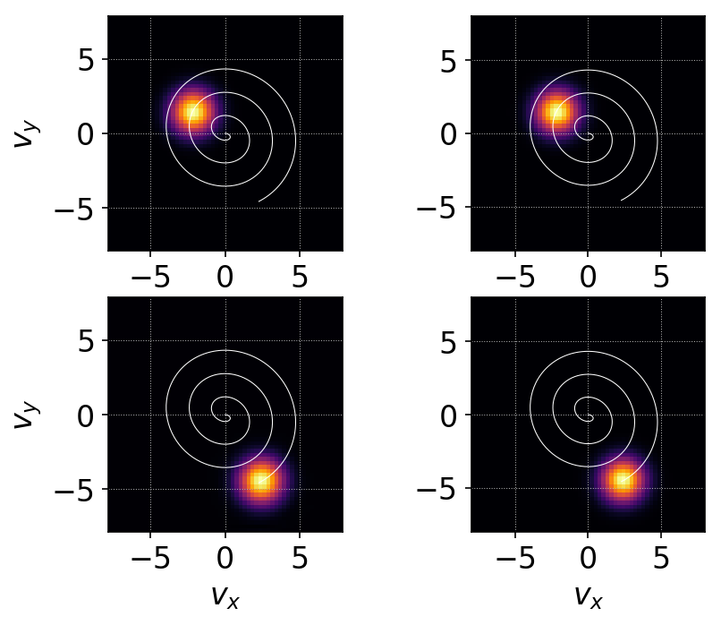
Comparison of Gkeyll distribution function (left column) and exact distribution function (right column) for test-particles in a oscillating electric (but uniform) field. Resonant case. Magnetic field is constant. The white line is the phase-space orbit starting at \(v_x=v_y=0.0\). The orbit is a spiral and the solution is a drifting Maxwellian. This plot shows that Gkeyll solutions compares very well with the exact solution. See vlasov-test-ptcls/c3 for input file.
A more quantitative comparison can be made by plotting the drift velocities from the simulation and the exact result. This plot is shown below.
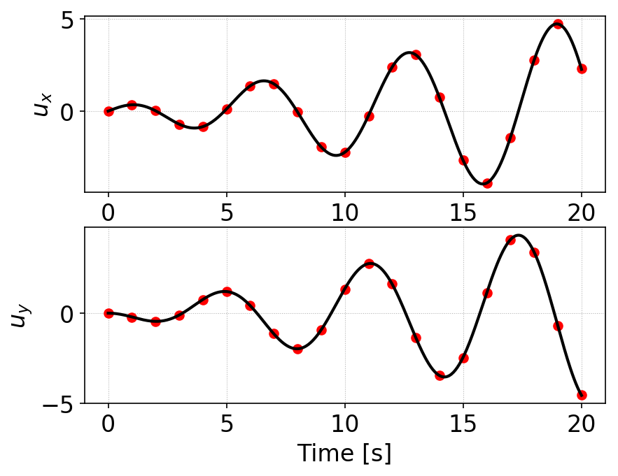
Comparison of x-component (top) and y-component (bottom) of drift velocities from simulation (red dots) with exact solution (black lines). The Gkeyll solutions compares very well with the exact solution.
Time- and spatially-dependent electric field
Now consider the magnetic field is constant and pointing in the z-direction, \(\mathbf{B} = B_0 \mathbf{e}_z\). The electric field is given by
The motion of ions in this field are given by three coupled ODEs
where I am assuming \(q = m = B_0 = 1\). (This means that \(\omega\) is normalized to ion-cyclotron frequency and time is measured in its inverse).
To understand the behavior of this system I solved it numerically using a time-centered scheme. The plots below shows the Poincare plot of the extended phase-space \((v_x,x=0,t)\). The plots were made by evolving eight particles over a 1000 periods and then plotting a dot when the trajectory crosses the selected phase-space section (modulo \(2\pi/\omega\)).
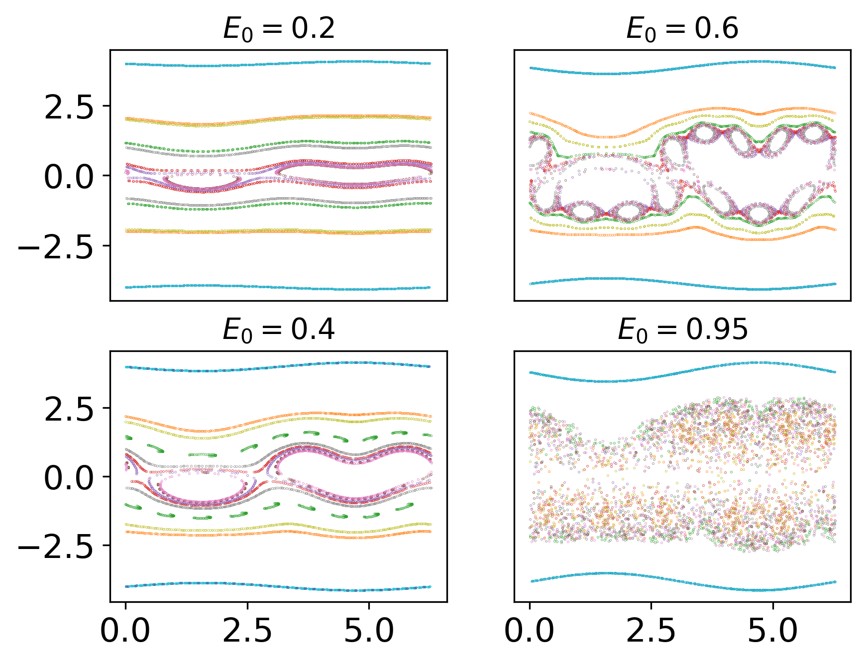
Poincare plots for test-particle motion in time-dependent electric field. The plots were made by tracing eight particles for hundreds of cyclotron periods. This figure shows that as the electric field strength increases the motion becomes stochastic. At first there are few island chains, which open up to form more island chains, eventually most low-energy particles become stochastic. Color indicate value of the distribution function carried by that particle. Given these plots one may conjecture that the distribution function will flatten when the particle orbits are fully stochastic.
Low-amplitude, non-stochastic case
First, consider \(E_0 = 0.5\) and \(\omega=0.4567\). In this low amplitude regime, the particle motion is regular. The domain is \([0,2\pi] \times [-6,6]^2\) and is discretized with a \(16\times 24^2\) grid, using polyOrder 2 Serendipity basis functions. The simulation is run to \(t=100\) with a Maxwellian initial condition with \(v_{th}= \sqrt{T/m} = 1\).
In this non-stochastic case we do not expect any significant heating of the particles. To diagnose this I plot the distribution function integrated over a single wavelength:
The following figure shows the integrated distribution function at four different times.
Integrated distribution function for time- and spatially dependent electric field case, at \(t=0\) (top-left), \(t=25\) (top-right), \(t=50\) (bottom-left) and \(t=100\) (bottom-right). This case has regular (non-stochastic) orbits and hence does not show any heating of the particles. Note that although the distribution function is non-Maxwellian the temperature has not changed significantly. See vlasov-test-ptcls/c4 for input file.
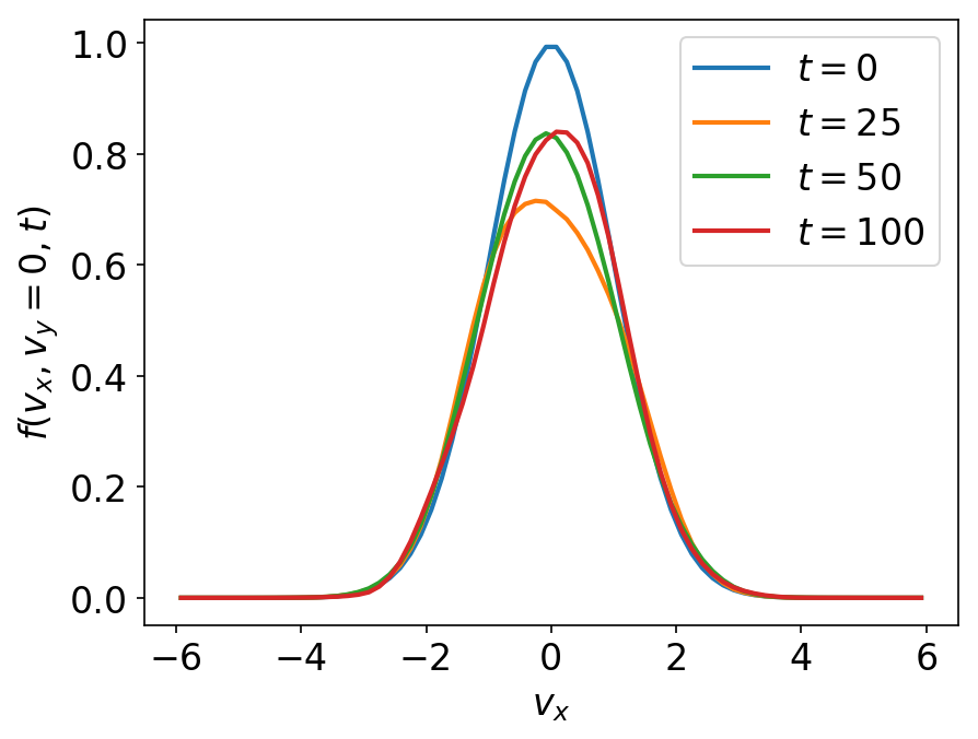
One dimensional line-outs of the 2D integrated distribution functions shown in the previous plot. The particles slosh around in the oscillating electric field, but the temperature has not changed significantly.
The thermal energy in the system, \(n v_{th}^2\) is shown below.
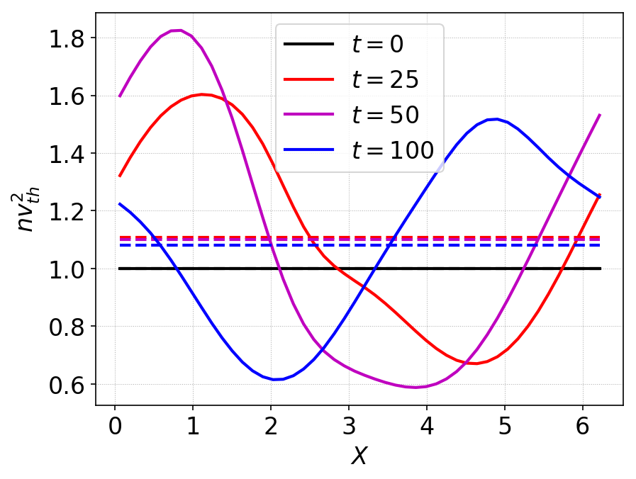
Thermal energy \(n v_{th}^2\) at various times. Dashed lines show the averaged thermal energy in the domain. This figure shows that the thermal energy only increases modestly (about 10%), indicating that the particles gains little energy from the fields.
Large-amplitude, stochastic case
Now consider \(E_0 = 0.95\) and \(\omega=0.4567\). In this large amplitude regime, the particle motion is stochastic. The simulation is run with the same parameters as the previous calculations.
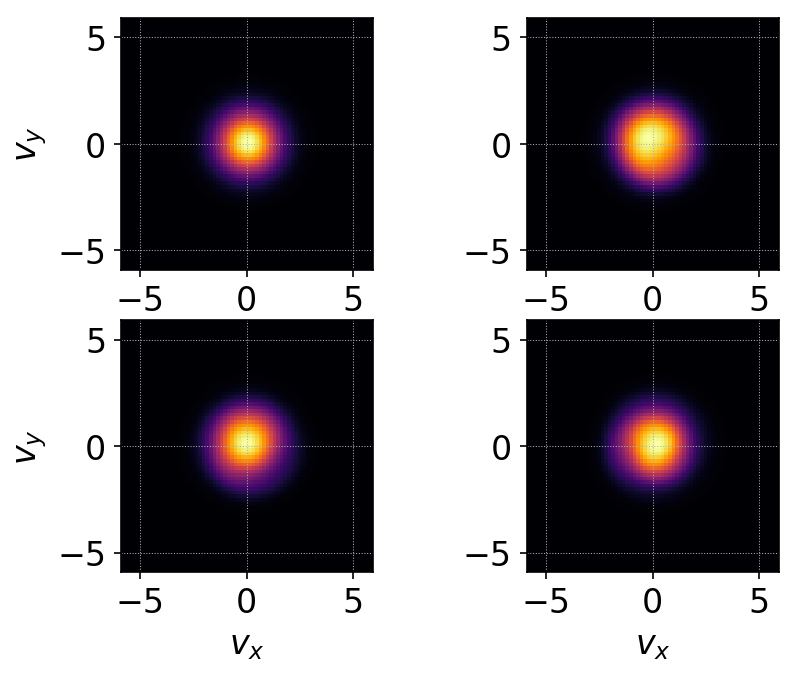
See movie of distribution function, showing \(f(x=\pi,v_x,v_y)\) and \(f(x,v_x,v_y=0)\). Complex phase-space structure is seen and also temperature increase is evident.
The following figure shows the integrated distribution function at four different times.
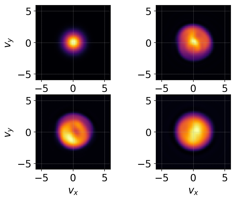
Integrated distribution function for time- and spatially dependent electric field case, at \(t=0\) (top-left), \(t=25\) (top-right), \(t=50\) (bottom-left) and \(t=100\) (bottom-right). This case has stochastic orbits and hence has significant stochastic heating of the particles. See vlasov-test-ptcls/c5 for input file.
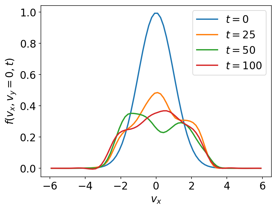
One dimensional line-outs of the 2D integrated distribution functions shown in the previous plot. The distribution function is significantly non-Maxwellian, showing flattening from stochastic heating.
The thermal energy in the system, \(n v_{th}^2\) is shown below.
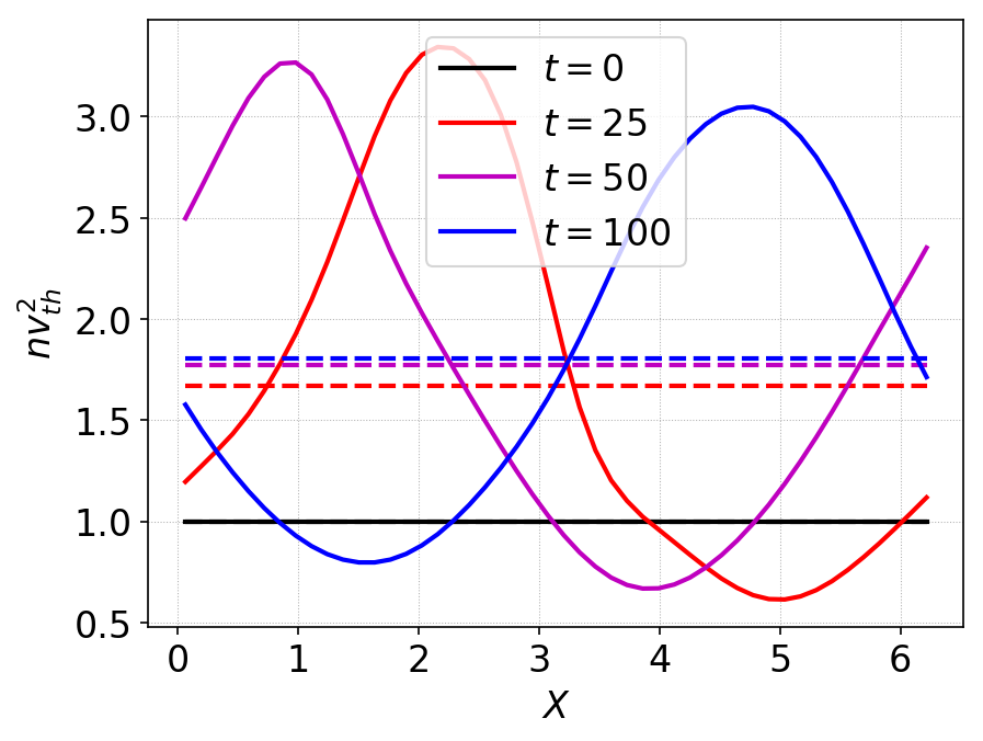
Thermal energy \(n v_{th}^2\) at various times. Dashed lines show the averaged thermal energy in the domain. This figure shows that the thermal energy increases significantly (almost 80%), indicating that the particles gain significant energy from the fields.
Conclusion
In this note I have tested some simple problems of test distribution evolution in specified electromagnetic fields. The code is first benchmarked against exact solution and then two cases of motion in a time-dependent field are studies. In the low amplitude regime the particle motion is regular, with little heating of the particles. In the large amplitude case the particle orbits are stochastic and this leads to significant heating, leading to flattening of the distribution function.
Questions: What are the signatures of stochastic particle orbits on the distribution function? Is it possible to develop Poincare type plots (or other unambiguous signatures) using the distribution function? Is there a self-consistent formulation, in which the distribution function feeds current to the fields? These topics will be explored later.