JE7: The dual Yee-cell FDTD scheme
Overview
The Finite-Difference Time Domain (FDTD) scheme uses the Yee cell to store the electromagnetic fields. The electric field components are stored on the corresponding cell edges, while the magnetic field components are stored on the corresponding face centers. See the following figure.
The advantage of the Yee-cell (and its dual) is that the discrete curl operators “move” the edge-based fields to the face centers and the face-based fields to edges. This provides a natural centering of the differencing operators, which when combined with a leap-frog time differencing leads to a second-order accurate scheme both in space and time. Further, the divergence relations are automatically satisfied [1].
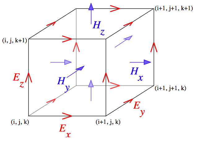
Standard Yee-cell. The electric field components are located on the edges while the magnetic field components are located on the face centers. In the dual Yee-cell the location of the electric and magnetic field components are swapped. Figure taken from Wikipedia.
The standard Yee-cell is usually preferred for most EM problems because it is easier to apply perfect electric conductor (PEC) boundary conditions. In certain situations, however, the dual Yell-cell is required due to constraints on the field locations from some other solves needed to study the physics. This is true for the two-fluid hybrid FV/FDTD scheme in which the current components are computed are face centers. In this note use Lucee to solve and test the EM equations on the dual Yee-cell (the standard Yee-cell was tested in JE6). This is in preparation of using this solve in a full two-fluid FV/FDTD divergence preserving scheme.
A note on the algorithms and boundary conditions
The FDTD method on the standard Yee-cell can be schematically written as
Here, the symbols \(\nabla_F\times\) and \(\nabla_E\times\) represent the discrete curl operators on face-located and edge-located fields respectively. For PEC boundary conditions the magnetic field components are copied on each of the lower boundaries, while the electric field components are set to zero on each of the upper boundaries.
The FDTD method of the dual Yee-cell can be schematically written as
For PEC boundary conditions the tangential electric field components are copied out on lower boundaries and the normal magnetic field components are copied on upper boundaries. Note that is not strictly necessary to apply the magnetic field BCs in this case as the normal derivative of normal field components never show up in the Maxwell equations. In addition, the electric field needs to be updated in one extra layer of cells on each upper boundary to ensure the correct update of the interior magnetic field.
Note that the order of updates in the two schemes is reversed, although the electric and magnetic fields are available at the same time levels.
Problem 1: 2D Transverse Magnetic modes in a box
This problem is identical to Problem 1: 2D Transverse Magnetic modes in a box. See that section for the initial and boundary conditions. The simulation was run on a \(80 \times 40\) grid and the electric field along the slice \(Y=20\) was compared to the exact solution. The results are shown below.
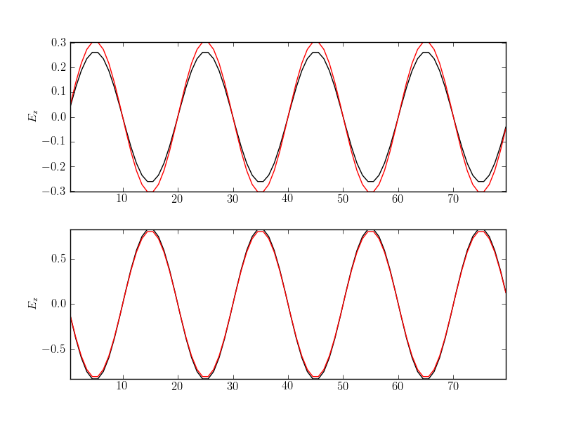
Electric field \(E_z\) along the slice \(Y=20\) as computed from the dual Yee-cell FDTD scheme (black) compared to exact solution (red) at \(t=75\) ns (top) and \(t=150\) ns (bottom). See [s63] for input file.
Problem 2: Electromagnetic pulse in a box
This problem is identical to Problem 2: Electromagnetic pulse in a box. See that section for the initial conditions and boundary conditions. The simulation was run on a \(100 \times 100\) grid and compared with a \(400 \times 400\) grid solution computed with the wave-propagation scheme. The results are shown below.
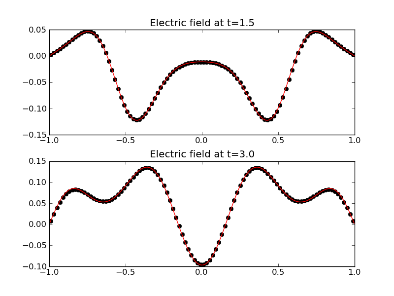
Electric field \(E_z\) along the slice \(Y=0\) as computed from the dual Yee-cell FDTD scheme (black dots) compared to converged solution (red) at \(t=1.5\) (top) and \(t=3.0\) (bottom). See [s64] for input file.
Conclusions
The FDTD scheme on dual Yee-cell is tested and shown to work correctly. One note (for the record) is that it took some time to get this algorithm to work correctly, specially the updates at the boundaries.