JE30: Solving the Hasegawa-Wakatani equations on overlapping domains
Note
This note is written in conjunction with Lee Ricketson of LLNL, and is part of the fusion exascale effort to produce a whole device gyrokinetic simulation of tokamak plasmas.
Introduction
Plasma dynamics occurs on a vast range of spatial and temporal scales. Often, specialized tools are developed to study one aspect of plasma physics, treating other aspects using simplified models or boundary conditions. One way to reuse existing tools to simulate more complete physics is to couple solvers (codes) together, each solver working on a different region, the coupling between them provided by boundary or overlap conditions. In this note I test a particular coupling scheme on the Hasegawa-Wakatani (H-W) equations. See JE17 for details on the solution method for the H-W equations.
The Hasegawa-Wakatani (HW) system is a coupled set of equations for the plasma density and electrostatic potential that describe resistive drift wave turbulence. These can be written as
where \(\zeta\) is the vorticity, \(\phi\) the electrostatic potential, and \(n\) the perturbed number density. Also, \(\kappa = -\partial/\partial x \ln{n_0}\) is a constant density gradient scale-length, \(\alpha\) is the adiabaticity operator and \(\mu\) is a hyper-diffusion coefficient. Also, \(\{a,b\}\) is the standard canonical Poisson bracket operator. The electrostatic potential itself is determined by solving a Poisson equation
In these equations, \(\alpha\) is a constant, making the problem 2D. The goal of this note is to solve the H-W equations on two overlapping domains and compare the results with a global, single domain result. This will allow studying stability and effectiveness of proposed coupling schemes, giving guidance on how to proceed with the more complex case of coupling the two gyrokinetic codes together.
Coupling Scheme
There are several possible ways in which simulations running on two different (but partially overlapping) domains can be coupled. In this note I use the following coupling scheme:
The density and vorticity equations are solved on separate but overlapping domains.
The potential equation is solved on a single, global domain that is the union of the two domains on which the density and vorticity are evolved.
Obviously, one needs to somehow couple the two domains to simulate the physics consistently. Call the left domain \(D_L\), the right domain \(D_R\) and the global domain \(D_G = D_L \cup D_R\), and the overlapping region \(D_O = D_L \cap D_R\). Then, the coupling algorithm has the following steps: In each RK stage do
Evolve \(\zeta\) and \(n\) on \(D_L\) and \(D_R\) using local potentials. For this step, the ghost cells of each domain are filled with the appropriate interior values from the other domain.
From the updated vorticity compute a global vorticity that takes the left/right domain values in the non-overlapping region, and takes average values in the overlapping region.
Use this global vorticity to solve the Poisson equation to determine potential on \(D_G\).
“Split” this potential by copying data from the global field to local fields stored on each sub-domain.
For completeness: I use a piecewise quadratic Serendipity basis discontinuous Galerkin scheme to evolve the vorticity and number-density, and a \(C^0\) finite-element method to update the potential. For time-stepping I use a strong-stability preserving third order Runge-Kutta (SSP-RK3) scheme. The coupling is performed after each RK stage. Perhaps another option would be to couple only after each time-step but this seems like a reasonable choice for now.
The solution is assumed to be doubly periodic. Note that this means that the left/right domains couple at two boundaries: the interior overlapping boundary and the shared boundary in the periodic direction. The overlap conditions and overlap averaging is performed by different updaters. This allows testing various sequence of steps directly in the Lua script by calling these updaters in different orders.
Results: Noise-free coupling scheme
In this first set of tests, results from a coupled simulation is compared to the single domain results. To ensure that the only errors are due to coupling, I force both the simulations to use the same time-steps. The global domain uses a \(32\times 32\) grid to discretize \(D_G = [40\times 40]\) box. The left domain uses \(20\times 32\) grid to discretize a \(D_L = [25\times 40]\) box, and the left domain uses \(16\times 32\) grid to discretize a \(D_L = [20\times 40]\) box. Note that the two domains overlap by 4 cells. A value of \(\alpha = 0.3\) is used for the adiabaticity coefficient. (Recall that \(\alpha = 0\) is incompressible Euler limit, and that \(\alpha \rightarrow \infty\) is the Hasegawa-Mima limit).
The coupling scheme in the case there is no interface noise (to mimic coupling errors) should give exactly the same results for the single domain and the coupled simulations. However, even small numerical roundoff errors in the sequence of steps (i.e. in finite precision, for example, operators that otherwise commute, don’t) can eventually add up, leading to a different turbulent realization. Note that for a turbulent simulation this is to be expected. What we want is to recover the statistical behavior, even though the exact realizations of the turbulent flow field may be different.
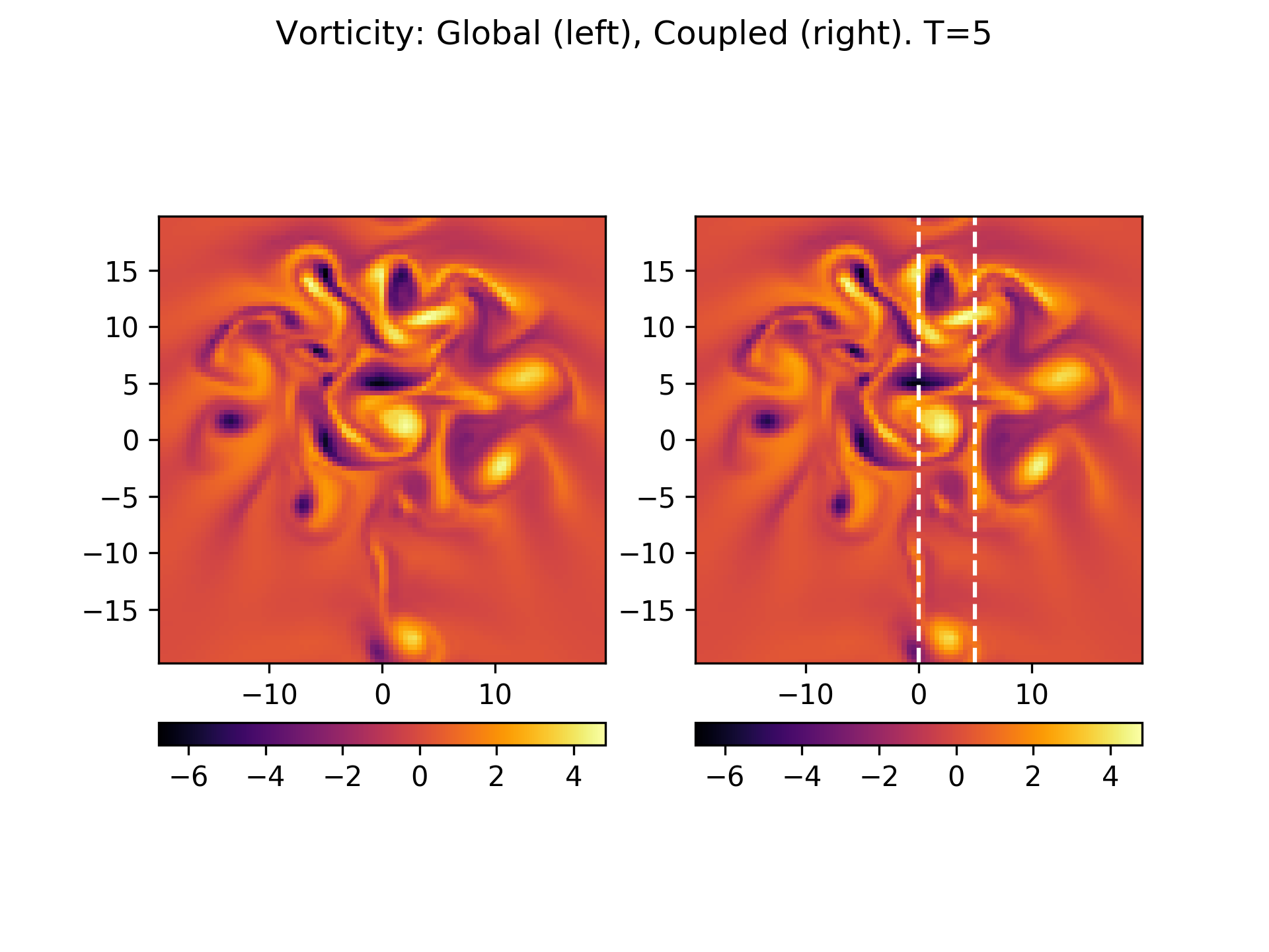
Early in time, drift wave turbulence is developing the global and coupled simulations produce identical results. See plot of vorticity below:

Vorticity at \(t=5\) from global (left) and coupled (right) simulations. White vertical lines represent locations at which coupling boundary conditions are applied, and the region between them is the overlap region. At this point, the global and coupled simulations give identical results.
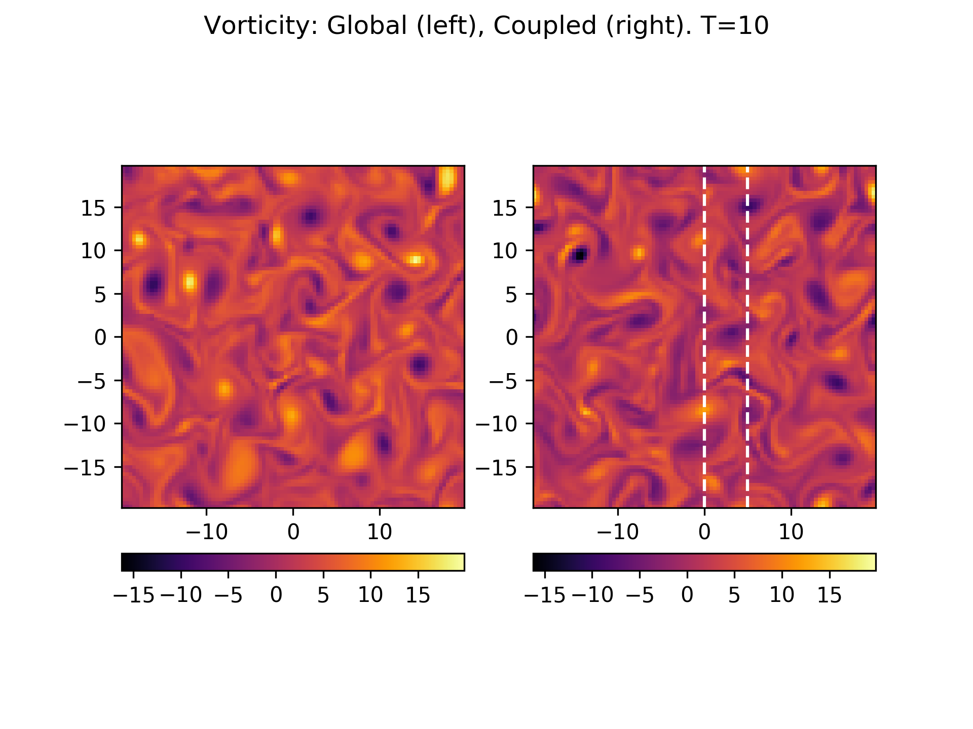
However, late in time when the system has become turbulent the solutions look visually different. See below:

Vorticity at \(t=10\) from global (left) and coupled (right) simulations. White vertical lines represent locations at which coupling boundary conditions are applied, and the region between them is the overlap region. At this point, the global and coupled simulations show different realizations of the flow, even though it appears that the two simulations have the same statistics.
Note that even though the results look different, it is hard to tell if this is really a problem. For turbulent flows, it is likely that any errors (even machine-precision errors) will eventually build up enough to lead to a different realization of the flow. The question we must ask: what are metrics for comparing results of turbulent flows? Perhaps one should look at time-average fluxes or turbulent spectra etc.
Results: 10% noise at coupling boundaries
In this set of calculations I add 10% random noise to the overlap condition: I pick a random number and use that to perturb the ghost cells values by 10%. This mimics (perhaps not very well) particle noise from a PIC solver. Note that the noise is grid-noise, i.e. has a spectrum peaked at high-k values.
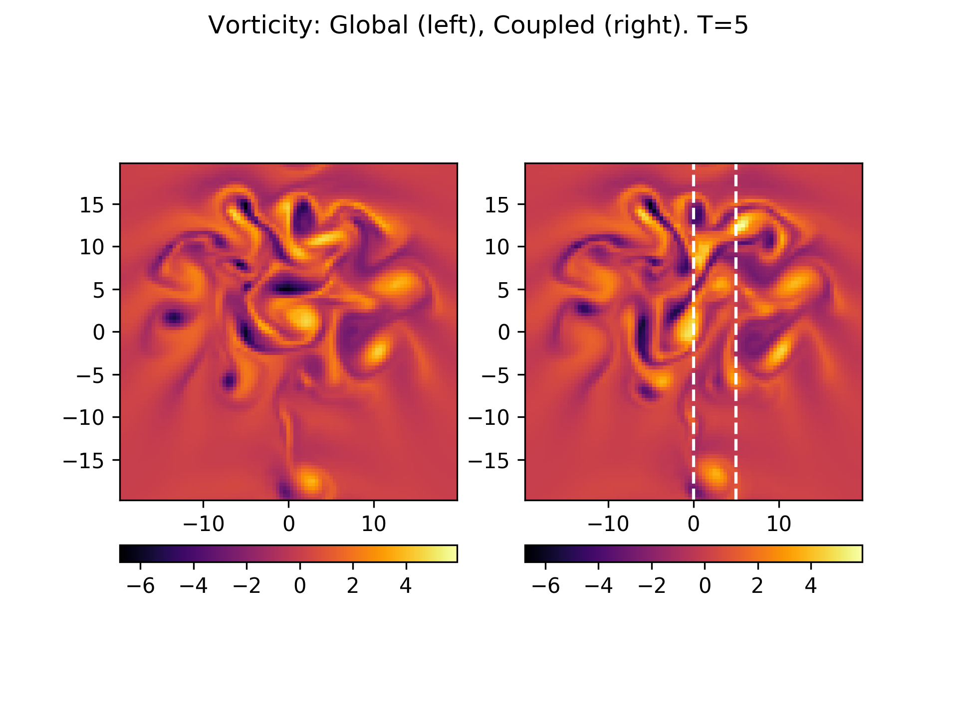
Due to the coupling noise in this case, even early in time the results between global and coupled simulations are different. See plot of vorticity below:

Vorticity at \(t=5\) from global (left) and coupled (right) simulations. White vertical lines represent locations at which coupling boundary conditions are applied, and the region between them is the overlap region. Even though early in time, the random perturbations lead to different realizations of the flow.
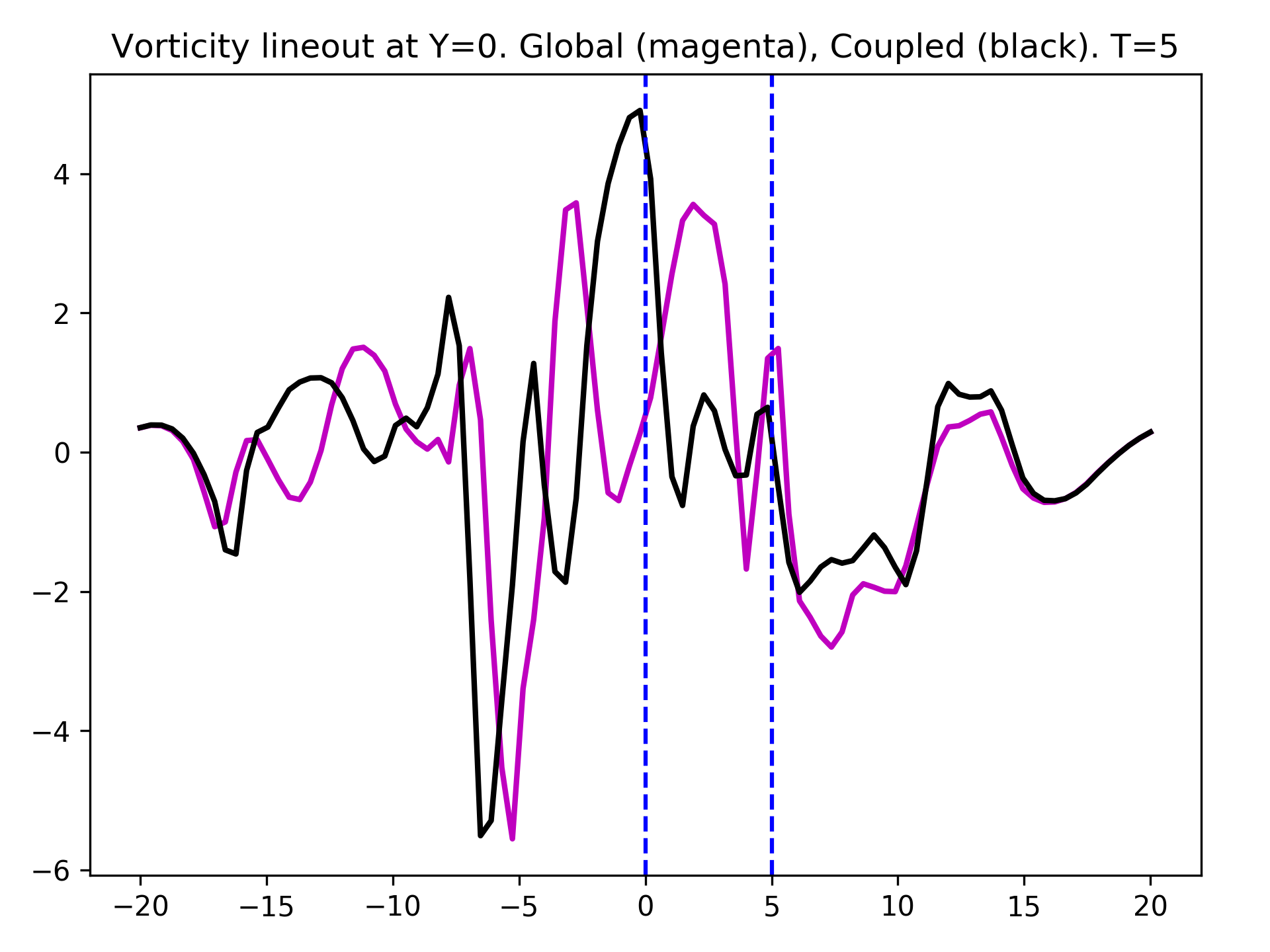
A lineout of the vorticity across the domain at \(Y=0.0\) shows the differences in the solution more clearly:

Lineout of vorticity at \(t=10\) from global (magenta) and coupled (black) simulations. Blue vertical lines represent locations at which coupling boundary conditions are applied, and the region between them is the overlap region. The global and coupled simulations show different realizations of the flow.
Late in time when the system has become turbulent the solutions look visually different, but seem to be statistically similar. See below:

Vorticity at \(t=5\) from global (left) and coupled (right) simulations. White vertical lines represent locations at which coupling boundary conditions are applied, and the region between them is the overlap region. The random perturbations lead to different realizations of the flow.
Conclusions (provisional)
It seems that the coupling scheme is very robust, that is, even though the turbulent flow realization are visually different, the scheme does not blow up or go unstable in any other way. However, we should come up with some metrics to measure errors from coupling when the flow itself is turbulent. This will be case in the case of the gyrokinetic coupling also as the system is inherently turbulent.
Solving the potential equation globally may not be the best way to move forward. Note that as the potential evolves in configuration space (and not phase-space) it is very cheap to update (compared to updating the distribution function). However, the software mechanisms to move number density and currents (and potential) between two codes onto/from a global mesh may be complex. Hence, an alternate approach might be to also solve the potential equations on local domains. I have not implemented this (yet) but will do so soon.
