JE18: Five-moment two-fluid reconnection on open domain

In this note I study the process of magnetic reconnection with the five-moment model. This model consists of a set of fluid equations for each of the species in the plasma (electron and ions in this case), coupled to the Maxwell equations via Lorentz force and currents. With a scalar pressure, the fluid equations can be written in non-conservative form as

\[\begin{split}\partial_t{n} + n \partial_j{u_j} + u_j \partial_j{n} &= 0 \\ \partial_t{u_i} + u_k \partial_k{u_i} + \frac{1}{mn}\partial_i{p} &= \frac{q}{m}\left(E_i + \epsilon_{kmi}u_kB_m\right) \\ \partial_t{p} + u_k\partial_k{p} &= -\gamma p \partial_k u_k\end{split}\]

where \(n\) is the number density, \(u_i\) is the fluid velocity, \(p\) is the scalar pressure and \(E_i\) and \(B_i\) are the electric and magnetic fields. The electromagnetic fields are computed by solving the full Maxwell equations.

Note

In the code the equations are solved in conservation-law form. The numerical scheme is a second-order finite-volume scheme, using a Roe approximate Riemann solver to compute numerical fluxes at cell interfaces to update the solution in a cell. The sources are handled using Strang splitting, and the source ODE is updated using a Crank-Nicholson implicit scheme. Positivity is ensured by switching to Lax fluxes and a first-order scheme on detection of negative pressure/density. This positivity fix occurs only very rarely, or not at all, and hence has negligible impact on the overall simulation accuracy.

The simulations are performed on an open domain, with the plasma initialized with a Harris current sheet with initial magnetic field given by

\[B_x(y) = B_0 \tanh{(y/L)}\]

where \(L\) is the current sheet half-thickness. With this initial magnetic field the conservation of total pressure (fluid plus magnetic)

\[p_e(y) + p_i(y) + \frac{B(y)^2}{2\mu_0} = \mathrm{const.}\]

can be used to determine the number density and pressure profiles (initial fluid temperatures are assumed constant). Using a background number density \(n_b\), this gives

\[n(y) = n_0\mathrm{sech}^2{(y/L)} + n_b\]

The other parameters are taken from [Daughton2006] as

\[\frac{\rho_i}{L} = 1,\quad \frac{m_i}{m_e} = 25,\quad \frac{T_i}{T_e} = 5,\quad \frac{\omega_{pe}}{\Omega_{ce}} = 3,\quad \frac{n_b}{n_0} = 0.3,\]

where \(\rho_i=v_{thi}/\Omega_{ci}\) is the ion gyroradius, \(v_{thi}=\sqrt{2T_i/m_i}\) is the ion thermal speed, \(\Omega_{cs}=e B_0/m_s\) is the species gyrofrequency and \(\omega_{pe} = \sqrt{e^2n_0/\epsilon_0 m_e}\) is the electron plasma frequency.

Picking a normalization as \(n_0=\epsilon_0=\mu_0=m_i=1\), gives \(B_0=1/15\), \(v_{the}=1/3\sqrt{6}\approx 0.361\), \(T_e = B_0^2/12\) and \(\rho_i=\sqrt{10/12}\).

Reconnection on a \(25d_i\times 25 d_i\) open domain

In the first set of simulations, the BCs are open (zero normal derivative of all quantities). The domain is \(25d_i \times 25d_i\), where \(d_i=c/\omega_{pi}\) is the ion inertial length.

Different grid sizes were used: \(256\times 256\), \(512\times 512\) and \(768\times 768\). This gives about 10 (20, 30) cells per \(d_i\) and 2 (4, 6) per \(d_e\), respectively. For a complete description of the simulation see the Lua program [s238].

Increasing the grid size reduces the numerical diffusion of the scheme, and shows qualitative differences in the current sheet structure. In the highest resolution runs (6 cells per \(d_e\), 30 per \(d_i\)) the electron diffusion layer is sufficiently well resolved and the simulation is assumed to be converged [1].

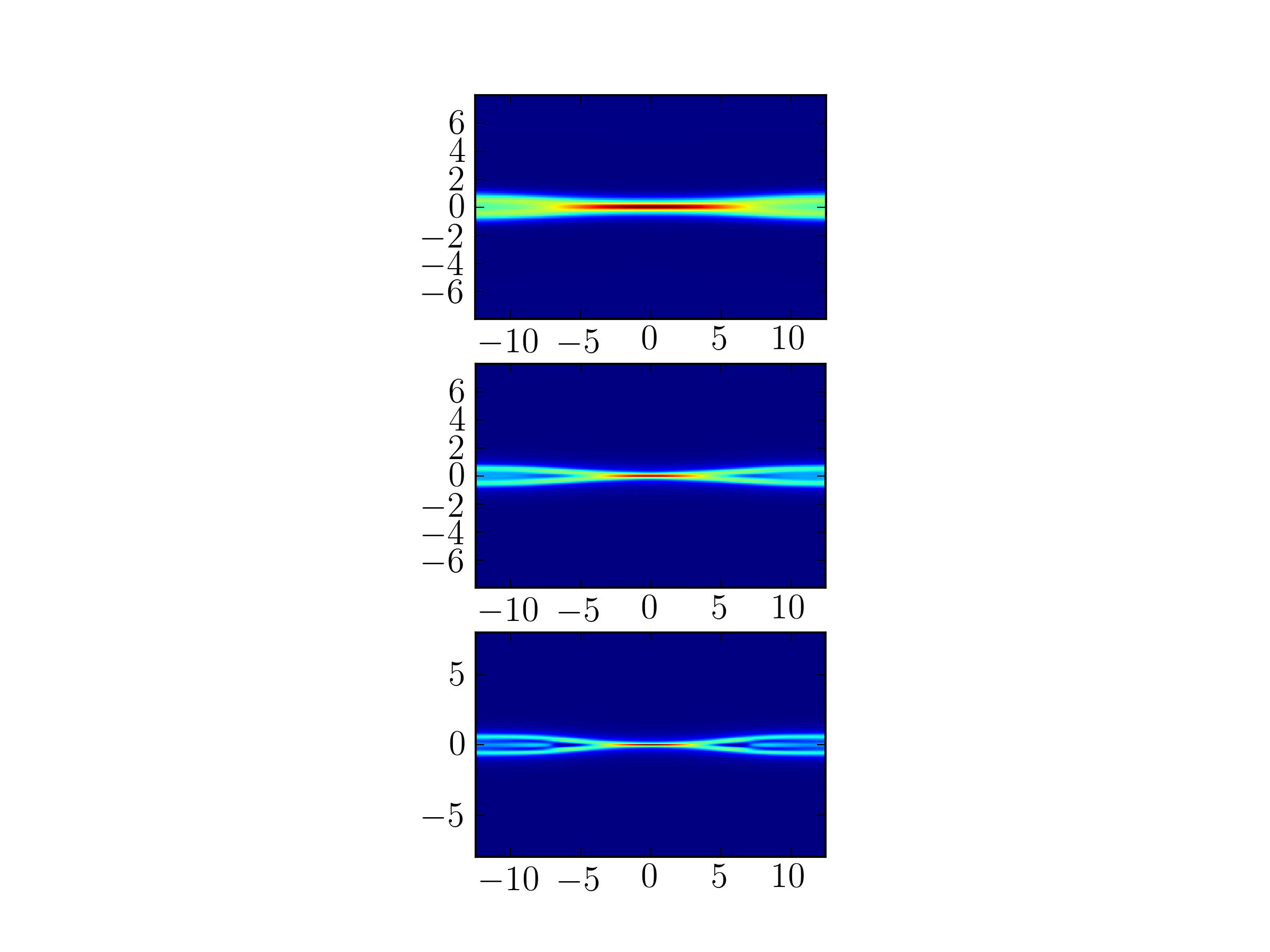
Electron out-of-plane current at \(t\Omega_{ci}=30\) with different grid resolutions. With 2 cells per \(d_e\) (upper), 4 cells per \(d_e\) (middle) and 6 cells per \(d_e\) (lower) respectively. The current sheet seems be getting thinner with increasing resolution, although the results do not significantly change in the lower two plots. See footnote [1] for caveats.

The set of plots below show the electron number density and \(B_x\) profile taken along a section \(x=0.0\) that passes through the X-point. The magnetic field upstream of the diffusion region (\(x\approx 3 d_i\)) is \(0.834\).

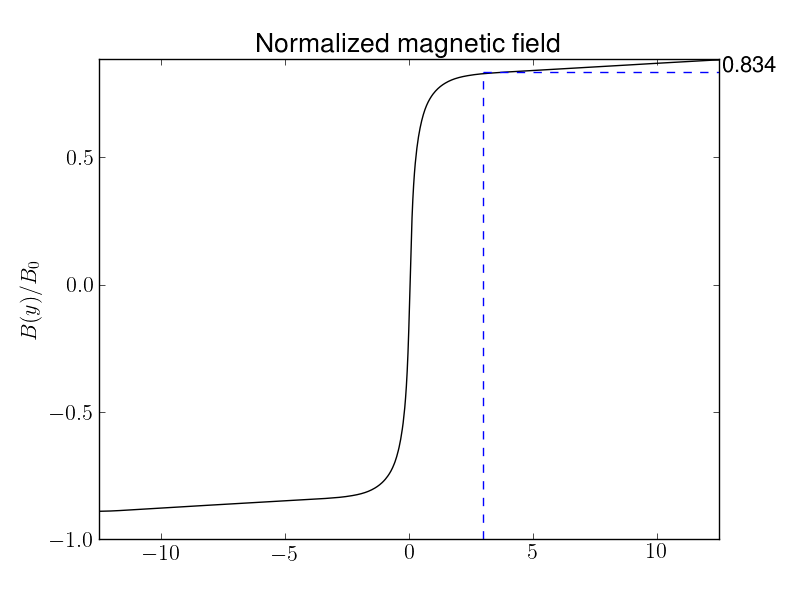
Number density (top) and magnetic field (bottom) along vertical slice at \(x=12.5d_i\). At the upstream edge of the diffusion region the magnetic field is \(B_x/B_0=0.834\). See [s238].

The set of plots below show the contours of various fluid quantities at \(t\Omega_{ci} = 30\). There is strong outflow in both the ion and electron fluids (on the order of \(0.5 v_{ti}\) and \(v_{the}\) respectively). The electron outflow velocity shows a strong flows along the current sheet, which then bifurcates along the magnetic flux separatrix. A careful look at the separatrix flow shows a reversal of the flow from outflow to inflow.

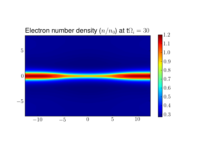
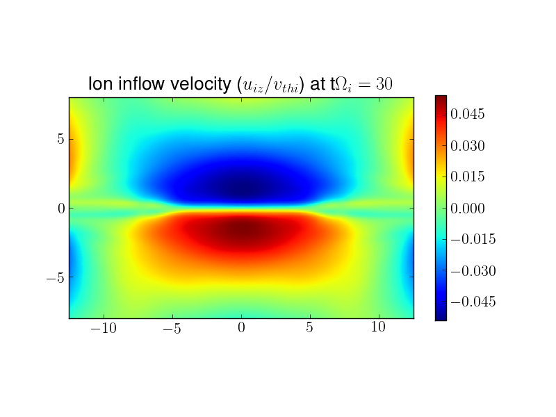
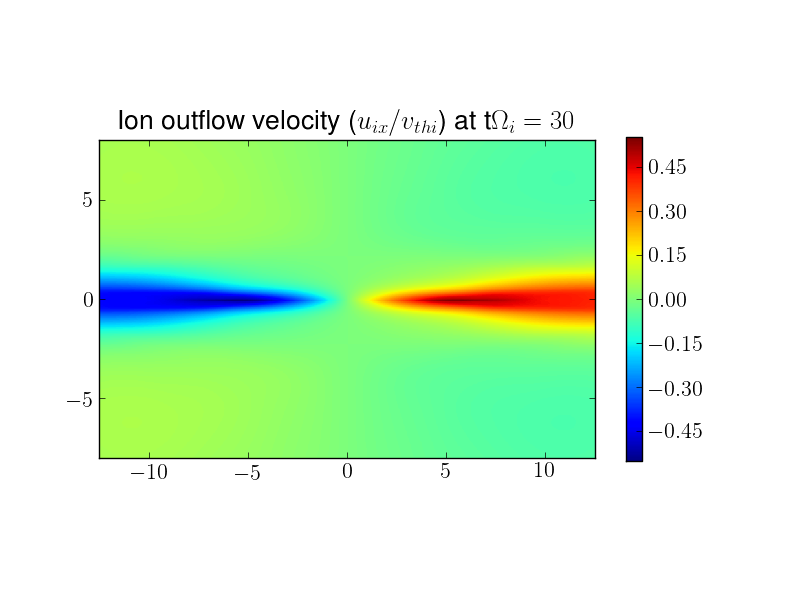
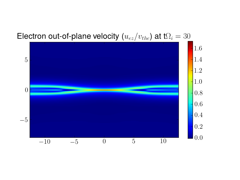
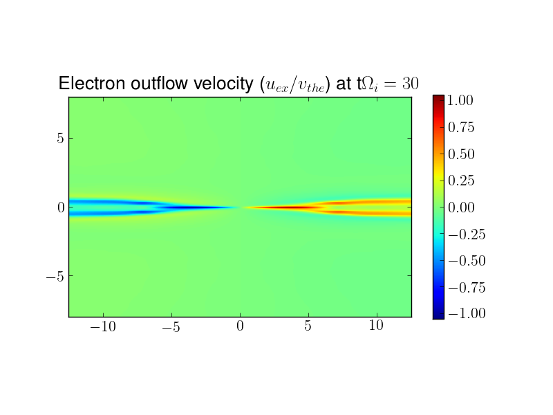
Number density, inflow ion velocity, outflow ion velocity, out-of-plane electron velocity and outflow electron velocity at \(t\Omega_{ci}=30\).

In the following plots the electron out-of-plane current is shown at \(t\Omega_{pi}=30\) and \(t\Omega_{ci}=45\). The current sheet is seen to elongate. Also seen are fluid jet instabilities (seen more clearly in the zoomed-in plot) which are formed due to the strong outflow of the fluids.

A movie of the electron out-of-plane currents can be seen here. This shows the formation of the current sheet due to reconnection, its elongation and the formation of jet instabilities due to the strong flow in the exhaust region.

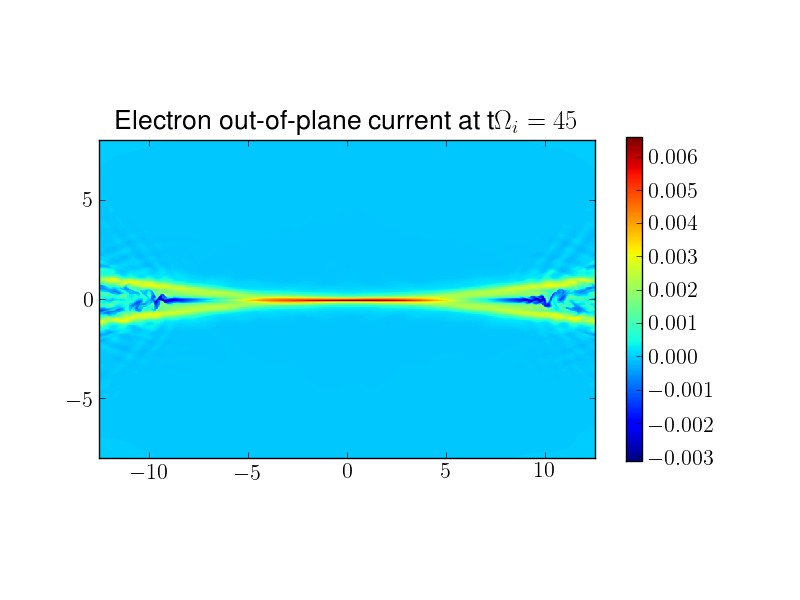
Electron out-of-plane current at \(t\Omega_{ci}=30\) and \(t\Omega_{ci}=45\). The reconnection current sheet is much thinner than the initial Harris sheet, which has half-width \(L\approx \rho_i\). The current sheet has elongated and jet instabilities are seen in the exhaust region due to the strong fluid outflow.

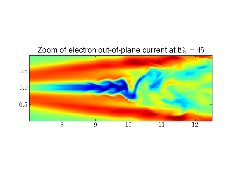
Electron out-of-plane current at \(t\Omega_{ci}=45\), zoomed in the right exhaust region. The fluid flow is unstable and shows vortices from the streaming of the fluid outwards into the exhaust region.

Conclusions

These initial studies of reconnection in open domains shows that the reconnection current sheet is much thinner than the initial Harris current sheet. In addition, rather unexpectedly (but also seen in the PIC simulation) the current sheet elongates late in time, extending nearly to the domain boundaries. Simulations with even bigger domains need to be performed to minimize the effect of the outflow boundaries on the current sheet dynamics. However, at this point it seems that the two-fluid five-moment model and the PIC model gives qualitatively similar results.

References

[Daughton2006]

William Daughton, Jack Scudder and Homa Karimabadi, “Fully kinetic simulations of undriven magnetic reconnection with open boundary conditions”, Physics of Plasmas, 13, 072101, 2006.

Footnotes

[1] (1,2)

This (convergence) is strictly true only if some sort of physical resistivity is included in the equations. The reason for this is that the ideal (without heat-flux and resistivity) two-fluid system has a large number of dispersive waves that will be captured as smaller and smaller scales are resolved. Some kinetic mechanism always damps such waves on a small scale. An extreme case of this “feature” is seen in shock simulations (see JE4) in which finer and finer scale structures are seen as the grid is resolved.

In numerical simulations damping is provided by numerical diffusion from the scheme. For physical correctness, some form of physical resistivity should be added, such that it damps out sub electron skin-depth structures.