JE38: Finite-Difference Schemes for Advection-Diffusion

Note

A description of the advection-diffusion equation, its properties and an overview on how to construct finite-difference methods to solve it is given in my class notes for AST560. Please see this link.

The complete code for the solver is in two files. Each individual simulation driver below is in its own C file. To build the code and the simulation driver download this zip file and type “make” in your terminal. Of course, for this to work you must have Gkyell installed. You do not need the complete Gkeyll source, just the core library. For building Gkeyll please see instructions on the Github page.

Introduction

The advection-diffusion equation is a fundamental equation that describes the transport of a scalar field \(f(\mathbf{x},t)\) in a given flow-field. We can write this as

\[\frac{\partial f}{\partial t} + \nabla \cdot (\mathbf{u}f) = \nabla \cdot (\alpha \nabla f )\]

Here \(f(\mathbf{x},t)\) is a scalar quantity, \(\mathbf{u}(\mathbf{x},t)\) and \(\alpha(\mathbf{x},t)\) are the (given) advection velocity and diffusion coefficient respectively. In many situations of interest the diffusion coefficient must be replaced by a diffusion tensor (a \(3\times 3\) matrix). This occurs when the diffusion is anisotropic, for example, due to the introduction of a prefered direction from a magnetic field.

This equation already contains the key features that arise in more complex systems. In fact, many fundamental kinetic equations are (nonlinear) advection-diffusion equations in phase-space. The nonlinearities arise as, in general, the advection velocity and the diffusion coefficient are functions of \(f\) itself. Here part we will see how to implement a finite-difference solver to evolve \(f(\mathbf{x},t)\) in a given flow-field. We will use this solver to understand the properties of the discrete scheme and to look at some interesting flows, including in phase-space.

On the Structure of the Solver

The solver implemented for this note is based on finite-difference methods. The advection is treated with either a second-order central scheme, or a first or third order upwing scheme. Upwinding, as we shall below, greatly improves quality of the solution. The diffusion is treated with either a second or fourth order central scheme. As there is not flow direction for diffusion central schemes are appropriate. The time-stepping is a SSP-RK3 stepper.

The solver works in 1D, 2D and 3D. The solver structure is simple: the normal component of advection velocity is evaluated at the middle of each cell face. This allows properly staggering the velocity at the face wehre the advective numerical flux is to be computed. The diffusion coefficient is evaluated at the cell centers: this is required as diffusion is computed using central differences. See Figure 7 of the notes. To choose the stencil to use we select the appropriate function pointer that implements the flux at a face given the cell-center values in two cells to the left and two to the right of that face. For example, the first-order updwing flux and the second order central fluxes are implemented by the functions

// First-order upwind
static inline double
calc_flux_upwind_1o(double vel, double fll, double fl, double fr, double frr)
{
  return 0.5*vel*(fr+fl) - 0.5*fabs(vel)*(fr-fl);
}

// Second-order central
static inline double
calc_flux_central_2o(double vel, double fll, double fl, double fr, double frr)
{
  return 0.5*vel*(fr+fl);
}

The function to use is then selected using a switch statement before the loop to compute the fluxes is performed. For example, for the advection update:

switch (app->a_scheme) {
  case ADV_SCHEME_C2:
    flux_func = calc_flux_central_2o;
    break;

  case ADV_SCHEME_U1:
    flux_func = calc_flux_upwind_1o;
    break;

  case ADV_SCHEME_U3:
    flux_func = calc_flux_upwind_3o;
    break;
};

The actual loop to update the fluxes is very simple: the outer loop is over directions and the inner over the faces (for advection) or cells (for diffusion). Using the dimensionally-independent looping and stencilling infrastructure in Gkeyll the same loop works for any dimension. The SSP-RK3 update is composed of three forward Euler steps. Each forward Euler step accumulates the advective and diffusive contributions and computes the maximum frequency (“CFL frequency”) that can be used to compute an estimate for the maximum stable time-step.

Advection of a 1D Gaussian

In the first set of problems a Gaussian distribution

\[f(x,0) = \exp(-x^2/\sigma^2)\]

where \(\sigma = 0.05\) is advected on a domain \(x \in [-1/2, 1/2]\) with advection speed \(u_x = 1.0\) to time \(T = 1.0\). The diffusion coefficient is set to zero. Results with two schemes are shown below: central difference and upwind. The simulation is implemented in the “cs-1d-guassian-advection.c” file.

In the central difference scheme one sees significant dispersion errors, though the \(L_2\) error is conserved. (The \(L_2\) error decays from the small amount of damping in the SSP-RK3 scheme as shown in the figure below). For the upwind scheme there remain dispersion errors, but much smaller. Of course, the \(L_2\) errors now decay due to the numerical diffusion from the upwinding.

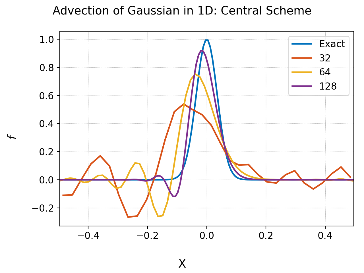
Advection of Gaussian in 1D with a second-order central scheme. There are significant dispersion errors that pollute the solution as the Gaussian propagates through the domain.

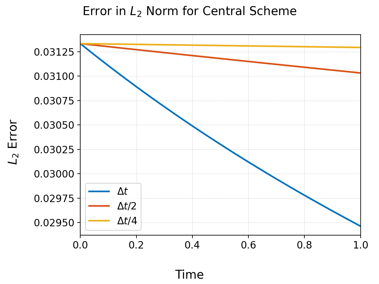
Advection of Gaussian in 1D with a second-order central scheme. The number of cells is held fixed to \(64\) but the time-step is reduced. The spatial scheme conserves \(L_2\) norm of the solution, but the SSP-RK3 scheme adds some diffusion. As the time-step is reduced the damping due to the time-stepper reduces with the order of the scheme.

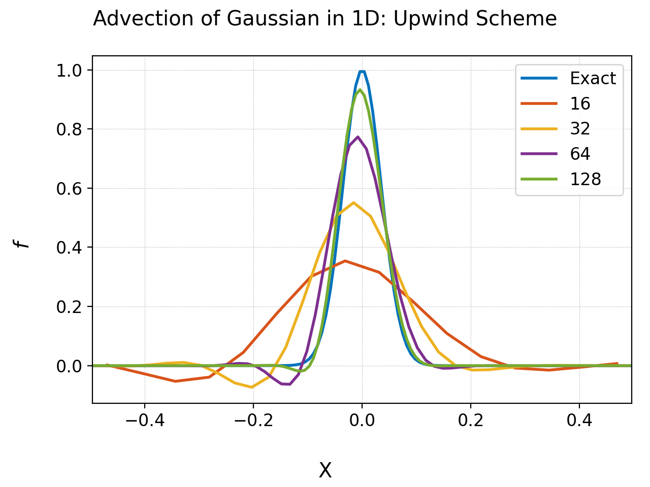
Advection of Gaussian in 1D with a upwind scheme. The dispersion errors are much smaller as compared to the central scheme, but still present. This indicates some form of limiters are required to reduce these errors further.

Rigid-body rotating flow

In this test a rigid body rotating flow is initialized by selecting the flow velocity \((u_x,v_x) = (-y+1/2, x-1/2)\) which represents a counter-clockwise rigid body rotation about \((x_c,y_c)=(1/2,1/2)\) with period \(2\pi\). Hence, structures in \(\chi\) will perform a circular motion about \((x_c,y_c)\), returning to their original position at \(t=2\pi\). See JE 12 for the same problem but with the DG scheme. The simulation is implemented in the “cs-2d-rotflow.c” file.

Two simulations were performed: one with central scheme and the other with upwinding. The diffusion was set to zero. The results are shown below. The central scheme shows more dispersion and phase errors than the upwind scheme. However, it is clear that neither schemes are not competitive with the DG scheme presented in JE 12. In general, this reflects the fact that the sub-cell resolution in DG allows greater control in designing schemes, allowing both greater accuracy and more efficiency, with much reduced dispersion.

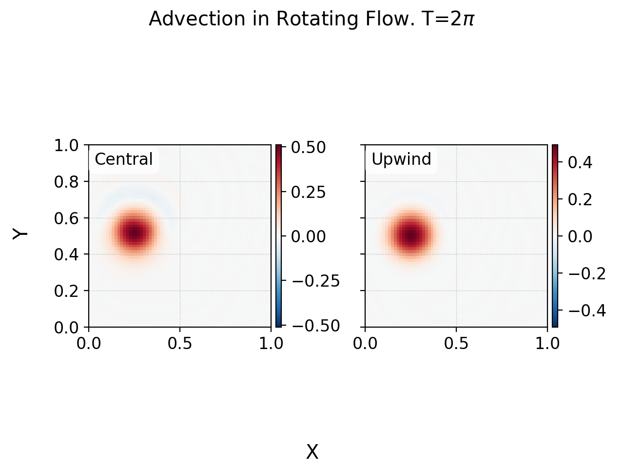
Advection of a blob in a rigid-body rotating flow. The blob has returned to its original position. Note the faint blue in the central difference result that shows dispersion errors. Such errors are also present in the upwind scheme, but are much smaller. See lineout plots below.

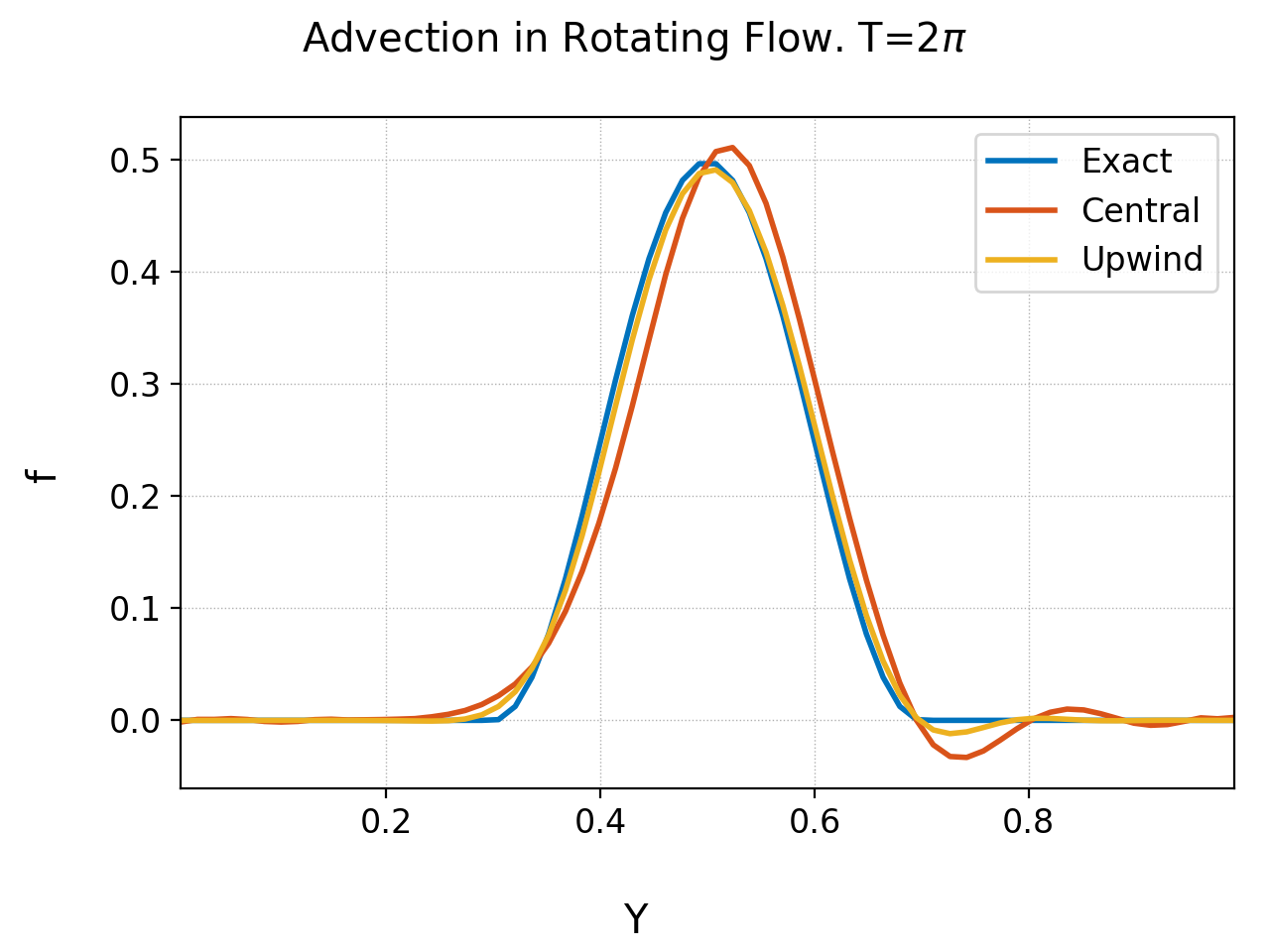
Advection of a blob in a rigid-body rotating flow. Shown is a lineout at \(x=0.25\). The blob has returned to its original position. The central difference scheme shows latger dispersion and phase errorss than the upwind scheme.

Charged Particles in a \(\cos(x)\) Potential

As we allow arbitrary flow velocity we can simulate the flow of particles in phase-space by initializing the advection velocity as the phase-space velocity of Vlasov equation. If we denote the domain by \((x,v)\) we set \(u_x = v\) and \(u_v = -\partial \phi / \partial x\), where \(\phi(x)\) is the electrostatic poential. For this test we set \(\phi(x) = \cos(x)\) and evolve a thermal distribution on a domain \([0, 2\pi]\times [-6, 6]\) on a \(64\times 64\) grid, with the thermal velocity set to \(1.0\). We use an upwind scheme with diffusion set to zero. The simulation is implemented in “cs-vlasov-cos-pot.c” file.

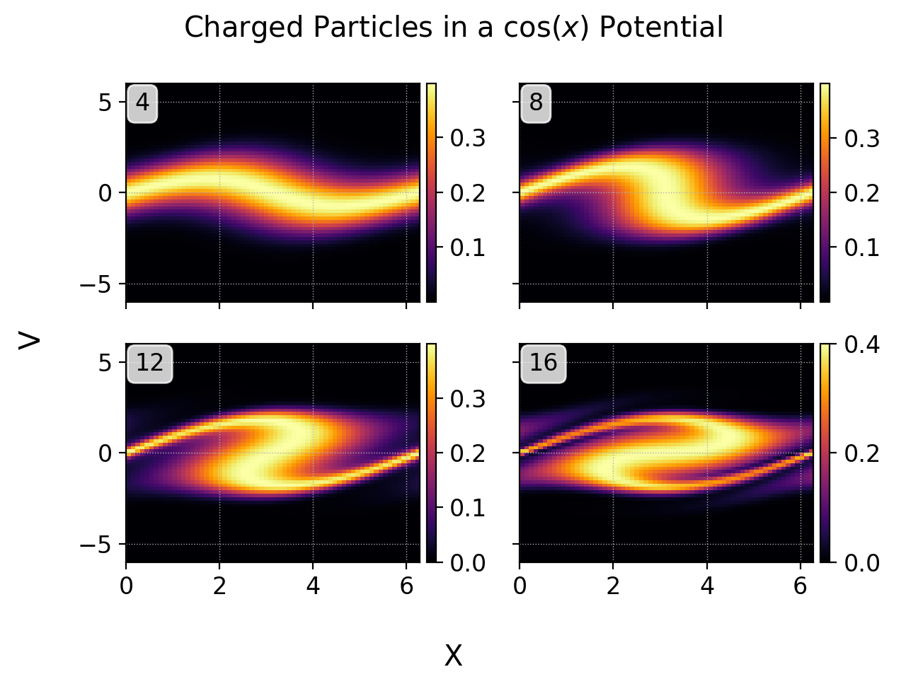
Charged particles advecting in a cos potential \(\phi(x) = \cos(x)\). Shown is the phase-space evolution of the distribution function \(f(x,v,t)\) at various times. Seen are the particles trapped in the potential well, with a passing particle population that are too energetic to be trapped.

Conclusions

We have shown how a simple advection-diffusion solver that allows setting arbitrary advection velocities can be used for many interesting problems, including advecting charged particles in a given electrostatic field. As advection-diffusion equations form the basis for a large class of kinetic equations that arise in plasma physics and other fields, extensions of these finite-difference schemes can be used to solve much more complex systems.

In general, however, we should mention that the disconinous-Galerkin schemes are far superior to the finite-difference algorithms presented in this note. DG schemes have natural sub-cell resolution that allows greater control on the scheme, and can give higher quality results on a relatively coarse mesh. Further, DG schemes are ideal for GPUs as the are FLOP-heavy, requiring only data in three cells, instead of a wide stencil as in high-order finite-difference methods presented above.